Published reports of field studies increasing require basic data on the climate of the study area. Much of the needed information is available from on-line data sources.
The routines in this section attempt to simplify the process of data extraction while maximizing the information gained from the data.
4.1 WHO Climate Station Data
There is a set of observation stations that record the daily weather. This is the WHO Climate Station Network.
Note
Note: This WHO observation network may not be the best one, for a number of reasons. However, the purpose of this report is to do a feasibility study of the output from a general climate data provider. If the products developed here have utility, the switch to a different data provider, if necessary, should be straightforward.
The purpose of this section is to show what stations are nearby a desired location, extract a period of data from a selected station, and then present visualizations and data that characterize the climate for the station.
In general, you only need to specify the geographic coordinates of a location. Defaults will select the nearest station, extract three years of daily values and present the results.
A map of the nearby observation stations is provided, along with some basic station information (e.g., elevation) just in case an alternative station is needed.
Similarly, the observation period can be changed. Warning: Be careful to choose a fairly short time interval (e.g., 5 years maximum) as daily data are extracted from the WMO database. An extended period will take a significantly long time to run and place unnecessary stress on the WHO server.
4.2 Library and Data Initialization
4.2.1 Caution
The code for these routines is not optimized as there are some on-going development efforts.
Show the code
## Standard packageslibrary(tidyverse) ## Handle datalibrary(lubridate) ## Handle date formatslibrary(gt) ## Create well-formatted tables## Specialized packages for maps## install_github("kimbridges/sitemaps")library(sitemaps) ## Loaded separatelylibrary(ggmap) ## Basemaps and Google Map key assistancelibrary(tidygeocoder) ## Used to reverse geocode to get country## Specialized packages## install_github("bczernecki/climate")library(climate) ## Support for meteo_ogimetlibrary(climaemet) ## Draws the Walter-Lieth climate diagramslibrary(plotbiomes) ## Whittaker diagramlibrary(sp) ## Point in polygon function## API keys## API keys are stored.column <-site_styles()hide <-site_google_hides()## Establish a theme that improves the appearance of a map.## This theme removes the axis labels and ## puts a border around the map. No legend.simple_black_box <-theme_void() +theme(panel.border =element_rect(color ="black", fill=NA, size=2),legend.position ="none")
4.3 Find the Climate Data Stations
The data come mostly from detailed records kept at airports and other significant government weather stations. In recent years, all of the data collection is automated. The source used here (ogimet.com) posts hourly data within about a day of its collection. We’re not using very recent data here, but this fact might be important in some study.
There are about 8,000 data collection stations. While there are many remote locations without nearby stations, the coverage is probably adequate for general uses. This is especially true in areas where the environmental gradients are shallow. Steep gradients are generally found associated with mountains.
The stations are grouped by country. That means it may be necessary to examine several adjacent countries to get a set of useful stations.
4.3.1 WHO Station Locations
Here is the general strategy.
Enter the longitude and latitude of a location that is central to your collections, or is a location in which you have a special interest. You can get this from Google Maps. Simply right click on a map location, left click on the geographic coordinates at the top of the pop-up window, then paste into your R code.
If your point is near a country border, you may want to enter a list of the countries that are in the general region. The default is to show only the stations in the country of your chosen location. If you enter a country name that has a blank in the middle (e.g., French Guiana or United Kingdom), you may need to put a plus sign instead of the blank (e.g., French+Guiana or United+Kingdom). Also, there are a few countries (e.g., Cambodia) that don’t have any entries.
If you want to search the database manually, go to ogimet.com.
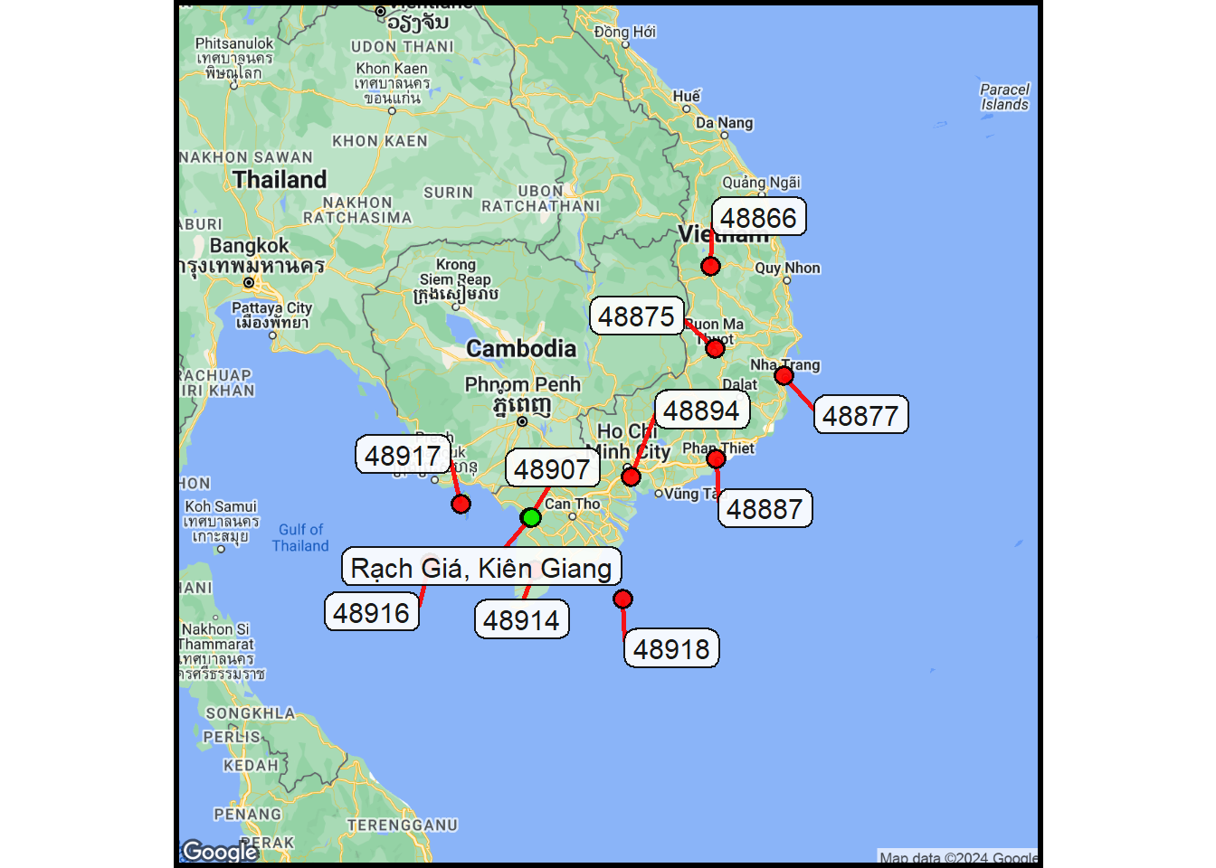
Here, you just put a location and let the system do the search. You get a list of the nearest 10 WMO stations and some useful characteristics of each station.
4.3.2 Special Case: USA
USA stations should modify the code and use nearest_stations_nooa (sic) function to extract the nearest station locations.
For all of the Hawaii stations, center on Honolulu and use
The lack of the + in the country above seems to be OK.
4.4 Enter Data Values
Here is where you enter the data. Note again that you probably only want to put in values for the lat and lon. Use decimal degrees.
There is usually no need to change any of the optional values, even though they look strange (e.g., stations <- 0). This is because this is the way that the use of default values is detected.
Show the code
## Required parameters. ## The location is all that is required to get info about WMO stations.lon <-105.1lat <-10## Optional parameters ########################################## ONLY CHANGE THESE IF YOU NEED A VALUE THAT IS NOT DEFAULT## Add a country list.## Example: country_list <- "Vietnam" or <- c("Guatemala","Belize")country_list <-""## Name the location of the (lat,lon) point. ## The format is 'text <- "put a name here"'.## Defaults to the area obtained with a reverse geocode.text <-NULL## Change the number of nearby climate stations (default=10).stations <-0## Change the number of years of climate data (default = 3).years <-0## Change the climate station numbe.## (defaults to the closest station).station_number <-NULL## Run weather data extraction from oligmet?## This is a slow process; don't repeat unless necessary (<- "no").## ORDINARILY THIS SHOULD BE LEFT AS "yes".run_extraction <-"yes"
4.5 Nearby Stations Located
The following chunks run without any changes or further input. Just leave the code alone and do run the chunk.
Show the code
## From here on, the processing is automatic when the chunks are run.## Process the data ################################### Create a data frame for the central locationcentral_location <-data.frame(lon, lat)## Find the country name.if(country_list =="") { ## Capture the country from the coordinates loc_info <-revgeocode(c(lon=central_location$lon,lat=central_location$lat)) country_list <-sapply(strsplit(loc_info, ", ", fixed=TRUE), tail, 1) } ## end country_list testcat("Full info about the site: ", loc_info,"\n\n")
Full info about the site: 248 Huỳnh Tấn Phát, P.Vĩnh Lợi, Rạch Giá, Kiên Giang, Vietnam
Show the code
## Extract the region fieldsregion <-sapply(strsplit(loc_info, ", ", fixed=TRUE), tail, 3)region <-paste0(region[1],", ",region[2])## Assign a site text instead of NULL.if(is.null(text)){ text <- region } ## end text checkcentral_location$text <- text## Use a default for the number of stations if not specified.if(stations ==0){stations <-10}## Apply the default for the number of years if not specified.if(years ==0){years <-3}## Format a table header.caption_info <-paste0("WMO Climate Stations centered on (", central_location$lat, ",", central_location$lon,")")## Get the nearby WMO stations.ns <-NULLns =nearest_stations_ogimet(country = country_list, point =c(central_location$lon, central_location$lat), no_of_stations = stations, add_map =FALSE)
## Rename some columns.station_info <- ns |> dplyr::rename(station = wmo_id) |> dplyr::rename(city = station_names)## Generate a table of the station information.gt(station_info) |>## Caption the tabletab_caption(caption = caption_info) |>## Fix the column labelscols_label(lat ="lat",lon ="lon",alt ="elevation",distance ="distance") |>## Format the numeric columnsfmt_number(columns =c(lat, lon), decimals =4) |>fmt_number(columns = distance, decimals =1) |>## Source Informationtab_source_note(source_note ="Source: Extracted using ogimet") |>## Footnotestab_footnote(footnote ="m ASL",locations =cells_column_labels(columns=alt)) |>tab_footnote(footnote ="km from central location",locations =cells_column_labels(columns=distance))
WMO Climate Stations centered on (10,105.1)
station
city
lon
lat
elevation1
distance2
48907
Rach Gia
105.0833
10.0000
3
1.9
48914
Ca Mau
105.1667
9.1667
3
93.8
48917
Phu Quoc
103.9667
10.2167
3
129.5
48894
Ho Chi Minh City-Nha Be
106.7167
10.6500
2
195.5
48916
Tho Chu
103.4667
9.2833
24
200.1
48918
Con Son
106.5833
8.7000
5
221.3
48887
Phan Thiet
108.1000
10.9334
8
352.5
48875
Banmethuot
108.0833
12.6833
537
450.2
48877
Nha Trang
109.2000
12.2500
10
524.7
48866
Pleiku City
108.0000
13.9834
801
552.8
Source: Extracted using ogimet
1 m ASL
2 km from central location
Show the code
## If not specified, assign the station number to## the first one (closest).if(is.null(station_number)){station_number <- station_info$station[1]}## Delete all the stations except for the station_number entry.station_info_one <- station_info |>filter(station == station_number)
Visualizing the locations may help.
4.6 Plot the Station Locations
Show the code
## Use the data from the previous chunk.## Reset the map defaults.column <-site_styles()## Rename the station column to meet the map requirement.s_info <- station_info |> dplyr::rename(text = station)## Build the basemap.basemap <-site_google_basemap(datatable = s_info)## Overlay the map with data points.## Show the map (with points & labels)station_map <-ggmap(basemap) +site_labels(datatable = s_info) +site_points(datatable = s_info) + simple_black_box## Change the point color.column$point_color <-"green"## Overlay the central location using the new color.station_map <- station_map +site_labels(datatable = central_location) +site_points(datatable = central_location)## Show the mapstation_map
It is a good idea to examine the list of WHO Weather Stations and the map with their locations with the question of whether the first one listed (it should be closest to the geographic coordinates you supplied) is the best one to use. Here are a few considerations:
Elevation: Is your location about the same elevation as the first station?
Distance: Are there other stations that are about the same distance that might be better in terms of data availability or reliability?
Data Quality: Are there reasons to suspect the quality of the data? (Later, there will be an evaluation of the amount of missing data.)
You can override the default station assignment (i.e., closest station) by providing a station number in the Data Input section and rerunning the code.
4.7 Extract the Climate Data
The data period begins and ends on year boundaries. The end is always the year prior to the current year.
The data are extracted from the database though the facilities of the climate package. This service is greatly appreciated.
As noted earlier, at this point, running the chunk does everything automatically.
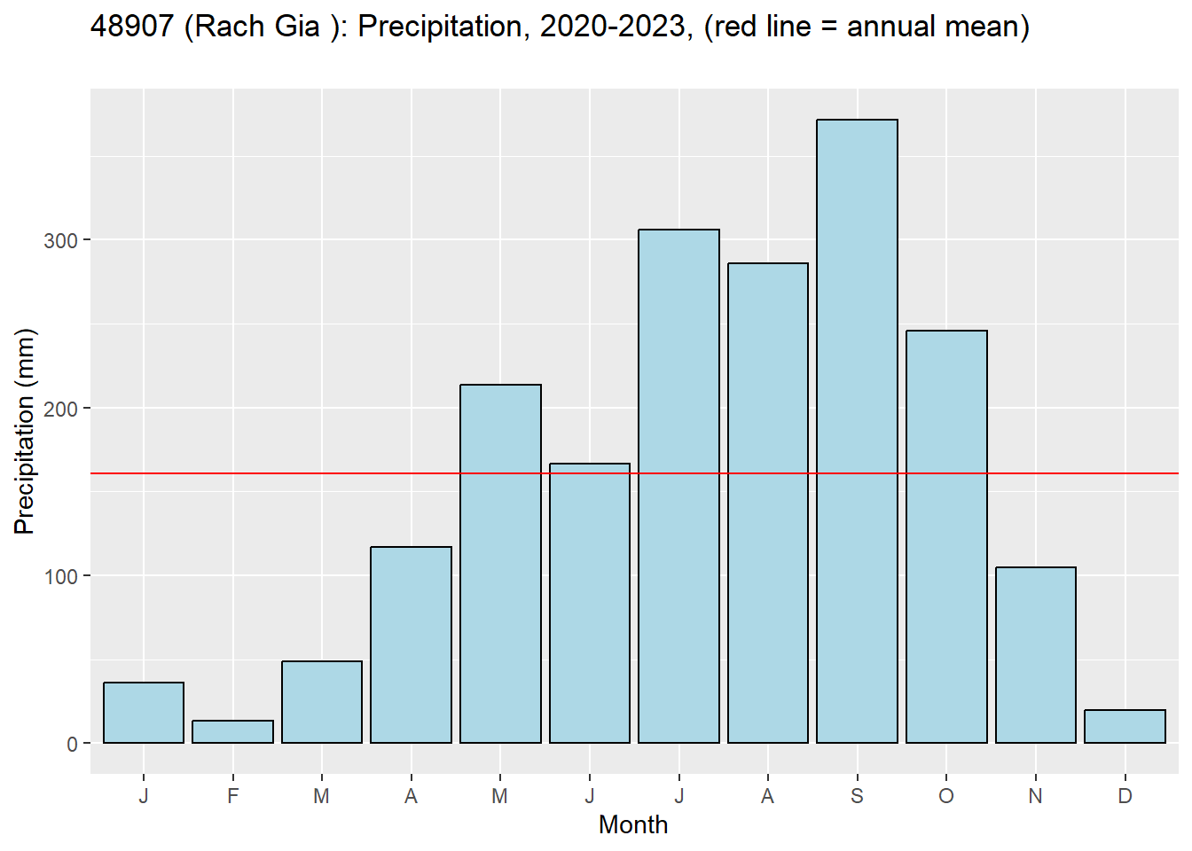
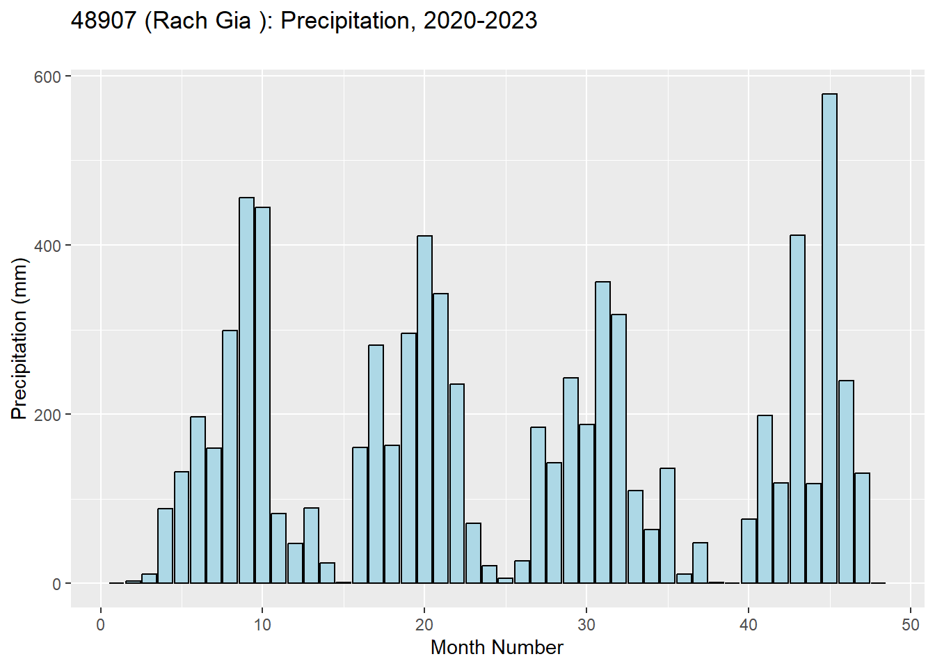
## PROJECT: MAKE THE X AXIS MONTH NAMES AND YEARSmonthly_trend_rain <-ggplot(monthly_trend) +geom_bar(stat ="identity", aes(x=month_count,y=m_rain_tot), fill="lightblue", color="black") +xlab("Month Number") +ylab("Precipitation (mm)") +ggtitle(paste0(place,": Precipitation, ",period_name,"\n")) monthly_trend_rain
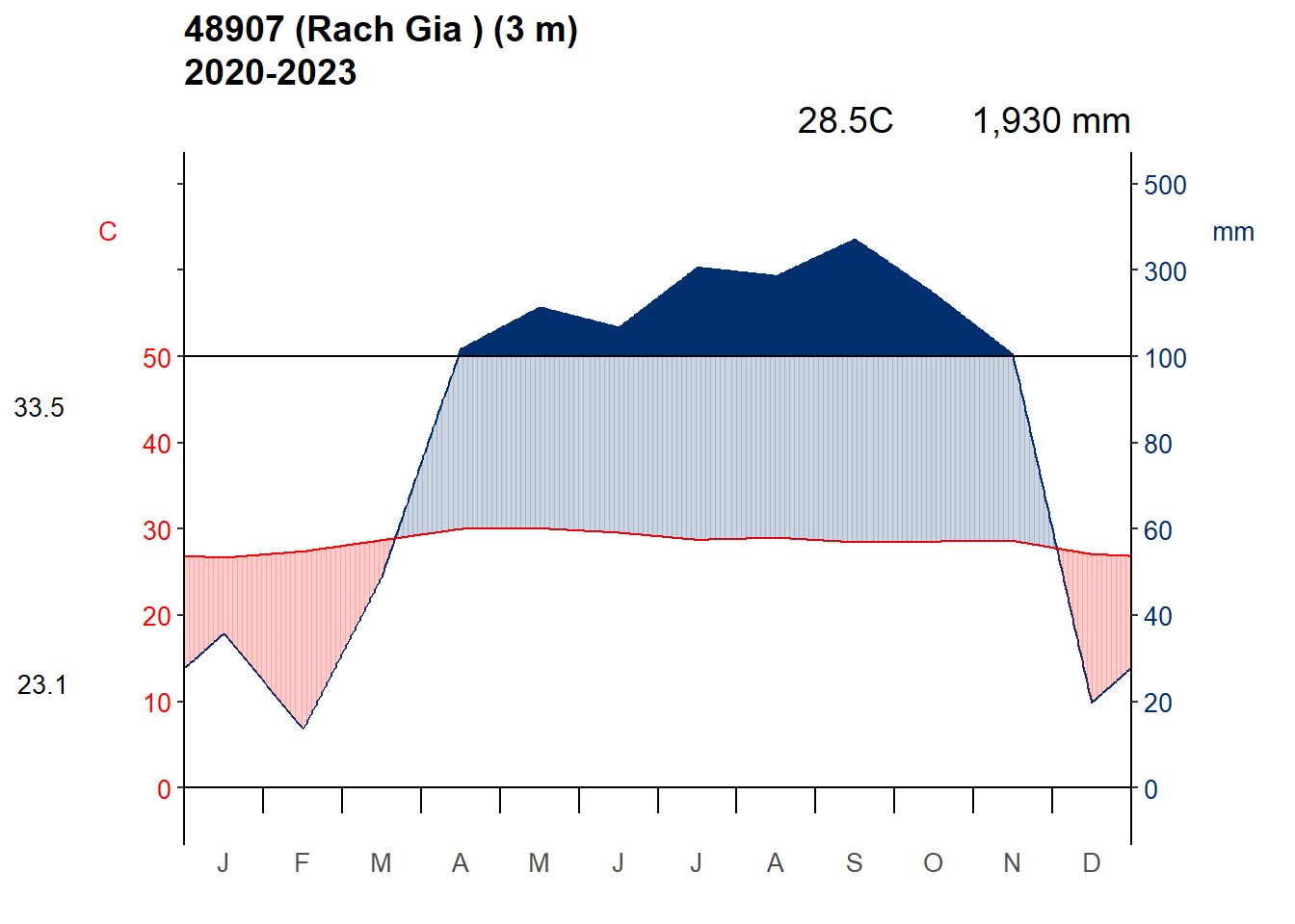
4.10 Climate Diagram
Show the code
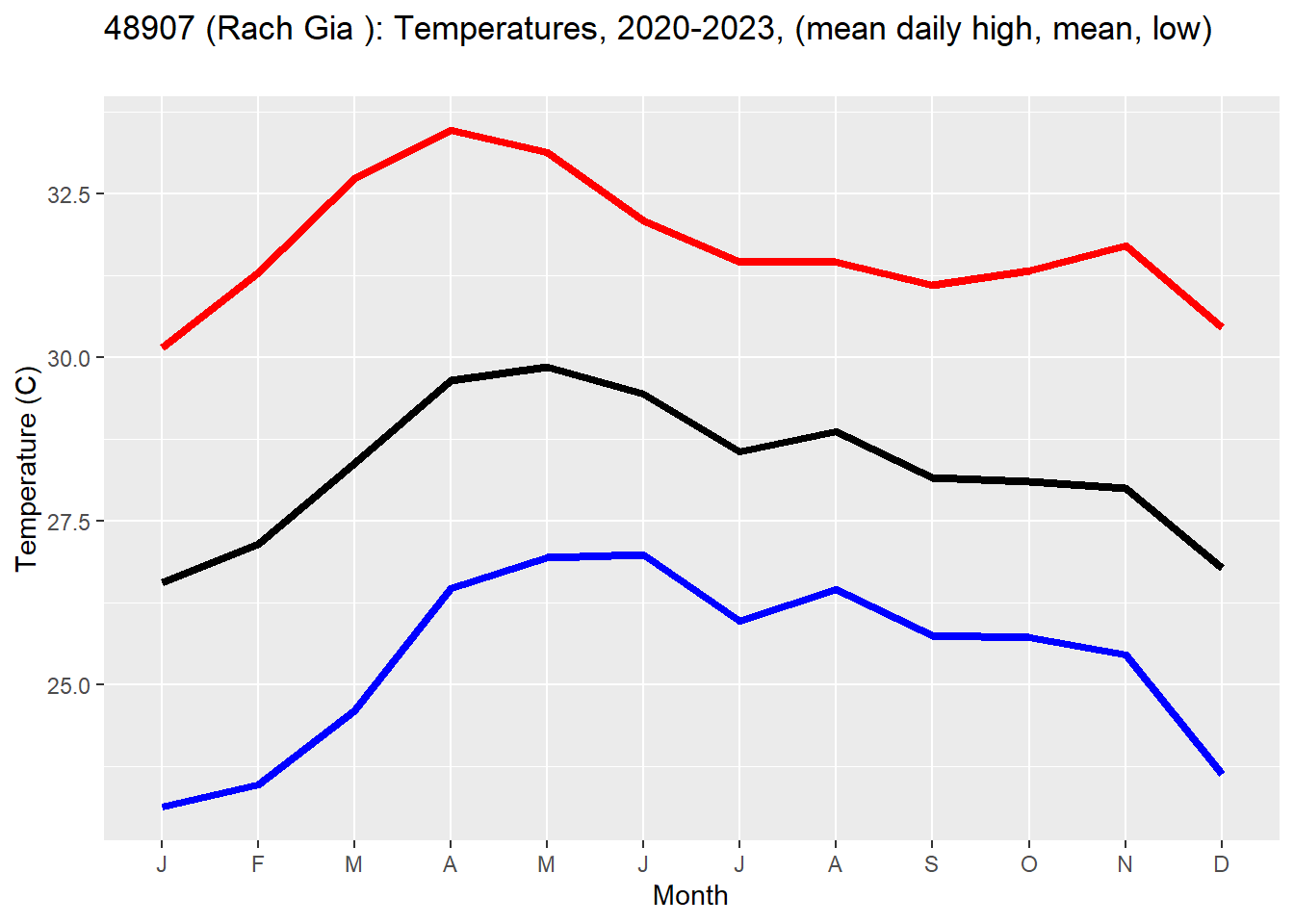
## Create a climate diagram.## Organize and name the data in a standard way.climate_data <- monthly_summary %>%select(m_avgrain_tot,m_avgmax_temp, m_avgmin_temp,m_minmin_temp) %>%rename(Ppt=m_avgrain_tot,Tmax=m_avgmax_temp,Tmin=m_avgmin_temp,Coldest=m_minmin_temp)## Transpose the data.climate_data_transposed <-as.matrix(t(climate_data))## This is a ggplot2 version of the diagwl function.c_diag <-ggclimat_walter_lieth(climate_data_transposed, mlab ="en", est = place, alt = station_info_one$alt, per = period_name, p3line =FALSE)## Show the plot.c_diag
Show the code
## Save plot in a file.ggsave(plot = c_diag, filename ="clim_diag.png")
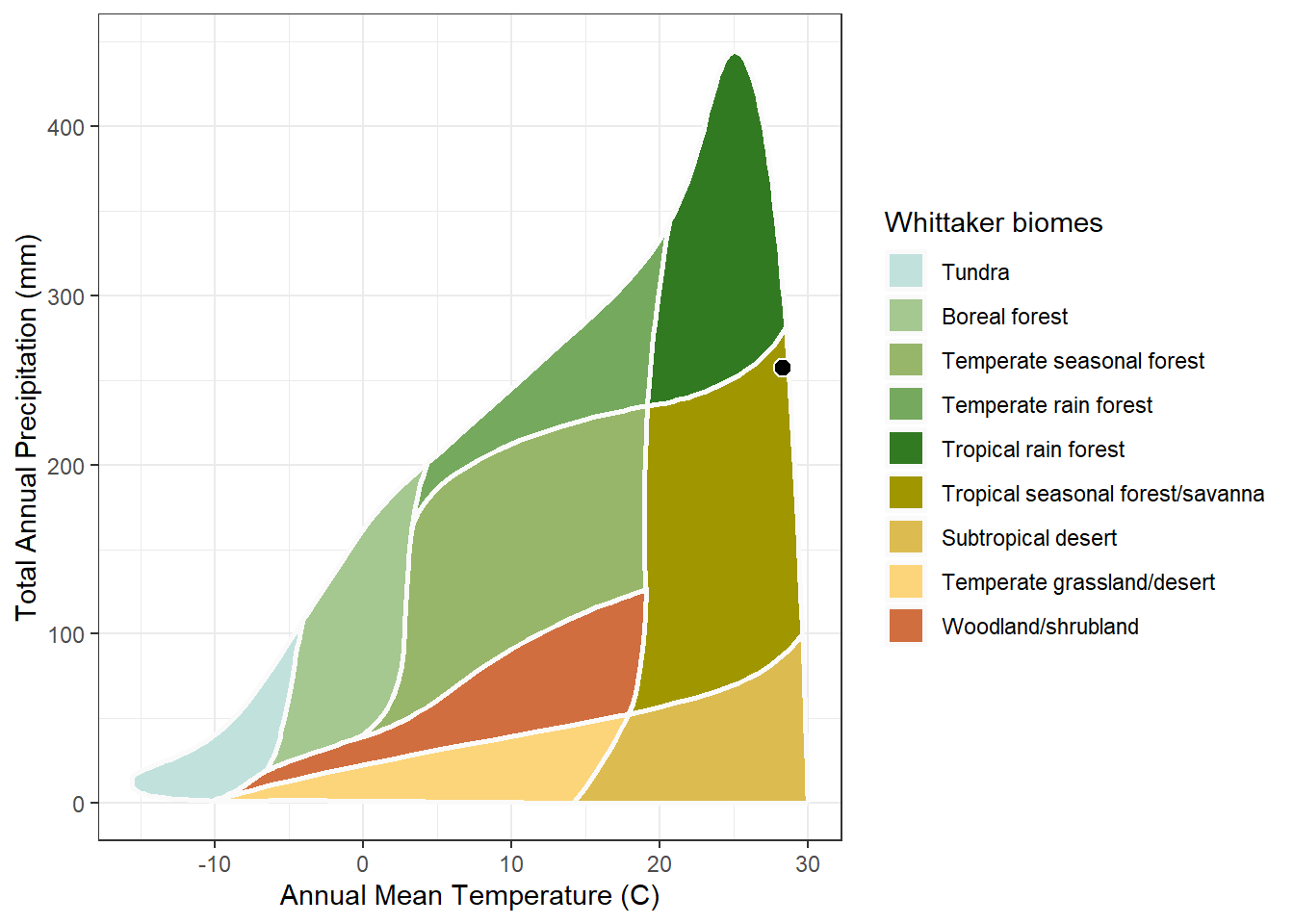
4.11 Biome Analysis
These functions determine the biome name and plot the location on a Whittaker diagram.
Show the code
############################################################name_biome <-function(mean_temp_c, total_ppt_mm){## Retrieves the biome name from the temp and prec.## requires dplyr, plotbiomes, sp biome_id <-NULL## Extract biome names. id <-unique(Whittaker_biomes$biome_id) biome_id[id] <-unique(Whittaker_biomes$biome)## Initialize the name (case: outside the diagram). biome_name <-"unknown"## Look inside each boundary for the point.for(i in1:9){## Isolate one of the boundary polygons (i.e., biome). boundary <- Whittaker_biomes |>filter(Whittaker_biomes$biome_id == i)## Test if the data point is inside the polygon. inside <-point.in.polygon(mean_temp_c, total_ppt_mm, boundary$temp_c, boundary$precp_cm,mode.checked =FALSE) ## If the point is inside, get the biome name.if(inside ==1){biome_name <- biome_id[i]} } ## End of boundary loopreturn(biome_name) } ## End function name_biome################################################################plot_biomes <-function(mean_temp_c =NULL,total_ppt_mm =NULL,source =NULL,label =NULL){## If no data points are given (e.g., mean_temp_c, total_ppt_mm),## you get just a basic plot of the Whittaker biomes.## Required libraries: ggplot, plotbiomes## Create the base plot. W_plot <-ggplot() +## Create the biome polygons.geom_polygon(data = Whittaker_biomes,aes(x = temp_c,y = precp_cm,fill = biome),# adjust polygon borderscolour ="gray98",size =1) +## Add axis labels.labs(x="Annual Mean Temperature (C)",y="Total Annual Precipitation (mm)") +## Use a better color scheme.scale_fill_manual(name ="Whittaker biomes",breaks =names(Ricklefs_colors),labels =names(Ricklefs_colors),values = Ricklefs_colors) +theme_bw()## Add data points if climate data are supplied. if(!is.null(mean_temp_c)) { W_plot <- W_plot +geom_point(aes(x = mean_temp_c, y = total_ppt_mm),size =3,shape =21,color ="white", fill ="black",stroke =0.7,alpha =1.0) } ## End of data point addition## Add label if label data are supplied. if(!is.null(label)) { W_plot <- W_plot +geom_label(aes(x = mean_temp_c, y = total_ppt_mm,label = label),color ="white", fill ="black",alpha =1.0,hjust =0, nudge_x =1.0) } ## End of label addition## Add caption at bottom if source is specified.if(!is.null(source)){ W_plot <- W_plot +labs(caption = source) } ## End caption additionreturn(W_plot) } ## End function plot_biomes################################################################## Obtain the name of the biome.name <-name_biome(mean_temp_c = mean_temp_c_annual, total_ppt_mm = tot_ppt_annual/10)paste0("The biome is: ",name,"\n")
[1] "The biome is: Tropical seasonal forest/savanna\n"
Show the code
## Plot just the biomes with a data point showing location.plot_biomes(mean_temp_c = mean_temp_c_annual, total_ppt_mm = tot_ppt_annual/10)