2  Exploring a Farmers Market

This is an exploration that uses a straightforward data collection technique to help understand the structure of a farmers market using the sale of produce by different vendors.

2.1 Generalizing the Process

The basic data consists of a grid that, in general terms, has species as rows and sites as columns. Inside the grid, a value of 1 means present and zero is absent.

This is a classic community-analysis table (generally called a “two-way table”).

There are many analysis situations in which the data are in this format. Here are a few examples (listed as row and column characteristics):

• Market Analysis: Produce and Farms or Vendors.
• Herbal Medicine Practitioners: Herbal species and Practitioners.
• Forest Plots: Trees and Sites.
• Menu Analysis: Menu items and Restaurants.

The point here is that the analysis structure laid out in this example is quite general. Only small modifications are needed in order to process the data for a study with this data structure.

The big difference, perhaps, is the process of getting data into the proper format. That’s where the LLM comes into play.

2.2 Analysis Structure

The data collection part of this analysis is quite straightforward. The analyses are, by comparison, complex.

The steps to do the analyses have been broken into “bit sized” modules to make the process relatively transparent. This structuring encourages verification of the analysis process, easy updating of the procedures and allows additional analyses to be added with relatively little effort.

2.2.1 Functions

A number of functions were developed to support the computations. These are found in a separate document.

Here is a list of the functions:

• read_lists
• species_list
• species_freq_plot
• site_freq_plot
• data_to_2way
• species_dendrogram
• site_dendrogram

The use of these functions simplifies the code shown here. The function code is loaded with a source function as part of the initialization.

2.2.2 API Keys

API calls use the resources of an external server. An example is the Google Map Server that’s used to create a map using the Google database. You need to (potentially) pay for this service. The mechanics involve getting an API Key from Google. This registers a credit card which will be used for payment.

The same general relationship holds for other API servers. The API keys used here are:

• Google Maps (for elevations, geocoding and map generation)
• Anthropic (for the Claude 3 LLM)

The actual keys are stored in the local computer system and not available for viewing.

2.2.3 Libraries and Data

There are quite a few packages that must be loaded. These are initialized, once loaded, with a library function. Some data and themes are also loaded as part of the initialization process.

## Set an option for the read_csv function
options(readr.show_col_types = FALSE) ## Suppress warning msg

## Standard Packages
library(tidyverse) ## Many useful functions
library(gt)        ## Tables
library(gtExtras)  ## Add functions to gt (tables)
library(readr)     ## read_csv function

## Specialized Packages
library(devtools)  ## Help install packages from github
## devtools::install_github("yrvelez/claudeR")
library(claudeR)   ## API access to Claude LLM
##devtools::install_github("rogerhyam/wfor")
library(wfor)      ## Species verification

library(sitemaps)  ## Draw maps
library(ggmap)     ## Create basemaps and more

library(googleway) ## Access to Google elevation
library(geosphere) ## 3D geometry calculations (e.g., distance)

library(ggdendro)  ## Dendrograms

## Get the API key.
claude_key <- Sys.getenv("ANTHROPIC_API_KEY")

## The "Lists" functions are under development.
## This loads the functions.
## You can see the functions in the "Functions" section of this document.
source(file="C://My_Functions/lists/lists_functions.R")

## Use two functions from sitemaps used to initialize column defaults.
column <- site_styles()
hide  <- site_google_hides()

## Establish a theme that improves the appearance of a map.
## this theme removes the axis labels and 
## puts a border around the map. No legend.
simple_black_box <- theme_void() +
              theme(panel.border = element_rect(color = "black", 
                                   fill=NA, 
                                   size=2),
                    legend.position = "none")

## Themes

dendro_theme <- function(){
  theme(
  panel.background = element_rect(fill = "lightsteelblue1"),
  panel.grid.major.y = element_blank(),
  panel.grid.minor.y = element_blank(),
  panel.border = element_rect(color     = "gray50", 
                              fill      = NA, 
                              linewidth = 0.7), 
  axis.ticks = element_blank(),
  axis.title.y = element_blank(),
  axis.text.y = element_blank())
  }

2.3 Testing Claude

The use of the Claude 3 LLM may not be possible due to being overloaded. This short module tests the availability.

## Test Claude 3 Opus
query <- "What is the capital of Botswana?"

response <- claudeR(prompt = list(list(role = "user", 
                                       content = query)), 
                    model = "claude-3-opus-20240229", 
                    max_tokens = 100,
                    api_key = claude_key)

## Note: A status code 529 means the server is overloaded.

cat(response)

The capital and largest city of Botswana is Gaborone. It is located in the southeastern part of the country, near the border with South Africa. Gaborone became the capital of Botswana in 1966 after the country gained independence from the United Kingdom. The city is named after Chief Gaborone, a local tribal leader. As of 2022, the population of Gaborone is estimated to be around 250,000 

2.4 The Study: Produce at a Farmers Market

This is a study that focuses on using an LLM (Large-Language Model) combined with R language code to analyze data that is typical in ethnobiology research.

2.4.1 Research Setting

Farmers Markets are magnets that attract ethnobiologists. It is in these local markets that researchers see the types of produce grown in a region. You don’t need to wander to remote places to find a farmers market. They are common everywhere.

2.4.2 Practice to Remove Productivity Barriers

It is common to collect data in a research study and then get stuck as other priorities delay the analysis and documentation of data. The lost momentum can be a significant factor in failing to complete a research study.

The code provided here attempts to reformulate the research process. It does this in several ways:

Collection: Data collection is streamlined by dictating observations using an unstructured, casual format.

Transcription: The dictation is converted to text automatically.

Extraction: Data are recognized in the transcription using AI technology. Data elements are extracted and formatted so they can be used without further intervention.

Processing: A standard set of analysis routines is run on the extracted data. This may include the automatic addition of data (such as elevations for locations) and the computation of new values (such as the distance between locations).

Visualization: A rich set of tables and graphic visualizations is produced to help in the verification of the data and the interpretation of the information.

2.5 Starting the Process

The data collection (i.e., dictation) and transcription aspects are not shown here. In summary, this is what is done with these two starting steps:

• Initialize: Start Google Docs on an Android phone. Press the microphone button on the keyboard.

• Tour: Walk through the market. Describe each produce vendor with the following three things:

  • Name: Some identifying name for the vendor.

  • Farm Location: A general location (e.g., city) where the vendor’s farm is located.

  • Produce: A list of items being sold by the vendor.

You can pause and restart the dictation. This is particularly handy when you use Google Docs and you may not need to stop the process (i.e., click the microphone button). Transcription will simply stop when you are not talking. When you are done, click on the check-mark icon, then give your document a name.

Your market description is now in the cloud. You can access it on a computer through the Google Doc web interface.

To use your text in this code, copy the document text into the R code, replacing the dialog text as shown below in the example.

2.6 Running the Analysis

The basic input data consists of information about the market (“location”) and a dialog that is the transcript of observations at the market.

Several request variables are provided that will give instructions to the LLM that should guide how the data are processed or to request additional information. There may need to be some modifications to these requests for dialogs that differ from the current example.

2.7 The LLM Requests

The coded requests are not easy to read. They are shown here for convenience.

2.7.0.1 source

Practice data (fake)

2.7.0.2 location

Farmers Market, in Torrance, California

2.7.0.3 dialog

I’m at the market and headed to the first vendor. The sign says Johnson Farms in Alhambra. All of the vendors come from California. This stand has a lot of tomato varieties, lettuce, broccoli, cabbage and chard. You could make a salad here. The next stand is Sato Brothers. They come from Fresno. That’s a long way away. Anyway, they’ve got watermelons, potatoes, and pumpkins. There are some food stands next. I’ll come back to these later. We’re now at Mountain Farm. The sign says Yucaipa. That’s up in the mountains for sure. Anyway, they mostly have apples and pears. There are some peaches, too. Next to them is Smith Orchards. It’s in Redlands. I didn’t know there are orchards there. The bins here are filled with fruit like oranges, limes and lemons. OK. There’s an Oceanside farm next. The name is Walter and Sons. It’s got lots of lettuce, tomatoes, cabbage and cauliflower. Another fruit farm is next. Let’s see. It says Riverside. And the name is National Fruit. That doesn’t sound very family farm like. Their specialty is oranges and lemons. Nakasone Farms is next. They’re found in Bakersfield. Their stand is selling lettuce, limes, apples, chard, and tomatoes.

2.7.0.4 request1

I need you to extract information from a story about a visit to a local farmers market. What I need are separate data rows. Each row should have only the name of a farm and a list of what produce they are selling with each item separated by a comma. Make sure to include all the produce being sold by each farm. Each produce item should be listed as singular. Just give the data lines as the response. Here is the story:

2.7.0.5 request2

Will you please extract the name of each farm, the city in which it is located and then add the latitude and longitude of the city. There should be just four decimal digits precision for these geographic coordinates and if the city is west of the prime meridian or south of the equator, the longitude coordinate value should be negative. The data should be presented in a csv-style table. The column names should be text, city, lat, lon. Please respond with only the table.

2.7.0.6 request3

You are an expert at finding the latitude and longitude of places. Will you please make a csv-like response, with no other comments, that has a column for the location, which is the name of the market, and it should have a column label text and the geographic coordinates with the column labels lat and lon. Here is the information you need:

2.7.0.7 request4

You know the proper scientific names of species of produce. I need you to convert a list of produce names to scientific names. The response should be in the form of a CSV style table without any other comments. This table should not include varieties. There also needs to be a column for the authorship of the scientific name. The columns should be labeled common, scientific, author. Here is the list.

2.7.0.8 request5

You are an horticultural expert on the market species found across Mexico. You know the most common local names, in Spanish, for the species you encounter in farmers markets. Your job is to add these local Spanish names to a table of species. Keep the table format in a CSV style with columns named ‘scientific’ and ‘spanish’. Respond with no other comments than the table.

## This is the information needed to run the analyses.

## The source of the data.
source <- "Practice data (fake)"

## The farmers market location.
location <- "Farmers Market, in Torrance, California"

## Transcript made at the market.
dialog <- "I'm at the market and headed to the first vendor. The sign says Johnson Farms in Alhambra. All of the vendors come from California. This stand has a lot of tomato varieties, lettuce, broccoli, cabbage and chard. You could make a salad here. The next stand is Sato Brothers. They come from Fresno. That's a long way away. Anyway, they've got watermelons, potatoes, and pumpkins. There are some food stands next. I'll come back to these later. We're now at Mountain Farm. The sign says Yucaipa. That's up in the mountains for sure. Anyway, they mostly have apples and pears. There are some peaches, too. Next to them is Smith Orchards. It's in Redlands. I didn't know there are orchards there. The bins here are filled with fruit like oranges, limes and lemons. OK. There's an Oceanside farm next. The name is Walter and Sons. It's got lots of lettuce, tomatoes, cabbage and cauliflower. Another fruit farm is next. Let's see. It says Riverside. And the name is National Fruit. That doesn't sound very family farm like. Their specialty is oranges and lemons. Nakasone Farms is next. They're found in Bakersfield. Their stand is selling lettuce, limes, apples, chard, and tomatoes."

## Instructions to extract the name, location and produce.
request1 <- "I need you to extract information from a story about a visit to a local farmers market. What I need are separate data rows. Each row should have only the name of a farm and a list of what produce they are selling with each item separated by a comma. Make sure to include all the produce being sold by each farm. Each produce item should be listed as singular. Just give the data lines as the response. Here is the story: "

## Instructions to extract locations of the farms.
request2 <- "Will you please extract the name of each farm, the city in which it is located and then add the latitude and longitude of the city. There should be just four decimal digits precision for these geographic coordinates and if the city is west of the prime meridian or south of the equator, the longitude coordinate value should be negative. The data should be presented in a csv-style table. The column names should be text, city, lat, lon. Please respond with only the table." 

## Instructions to get the location of the market.
request3 <- "You are an expert at finding the latitude and longitude of places. Will you please make a csv-like response, with no other comments, that has a column for the location, which is the name of the market, and it should have a column label text and the geographic coordinates with the column labels lat and lon. Here is the information you need: "

## Instructions to get scientific names of the produce.
request4 <- "You know the proper scientific names of species of produce. I need you to convert a list of produce names to scientific names. The response should be in the form of a CSV style table without any other comments. This table should not include varieties. There also needs to be a column for the authorship of the scientific name. The columns should be labeled common, scientific, author. Here is the list."

## Instructions to get common names in Spanish.
request5 <- "You are an horticultural expert on the market species found across Mexico. You know the most common local names, in Spanish, for the species you encounter in farmers markets. Your job is to add these local Spanish names to a table of species. Keep the table format in a CSV style with columns named 'scientific' and 'spanish'. Respond with no other comments than the table."

2.8 Use Claude 3 to Extract Information

The data will be processed to provide a basic set of information about produce vendors at the market.

The first step of to extract the data so that the data values are in a form that can be used with R programming.

Note that process from this point forward should be automatic as each chunk is run.

## Build the first query.
query <- paste(request1, "###", dialog, " ###")

## Submit the first query for processing.
data_rows <- claudeR(prompt = list(list(role = "user", 
                                       content = query)), 
                    model = "claude-3-opus-20240229", 
                    max_tokens = 2000,
                    api_key = claude_key)

data <- read_lists(data_rows=data_rows)

## Submit the second query for processing.
query <- paste(request2, "###", dialog, " ###")
data_rows <- claudeR(prompt = list(list(role = "user", 
                                       content = query)), 
                    model = "claude-3-opus-20240229", 
                    max_tokens = 2000,
                    api_key = claude_key)

data2 <- read_csv(file = data_rows)

## Submit the third query for processing.
query <- paste(request3, "###", location, " ###")
data_rows <- claudeR(prompt = list(list(role = "user", 
                                       content = query)), 
                    model = "claude-3-opus-20240229", 
                    max_tokens = 500,
                    api_key = claude_key)

data3 <- read_csv(file = data_rows)

2.9 Use the Extracted Information

The following chunks do different parts of the analysis. Consider this a step-wise approach. Check the results of each phase of the analysis.

2.9.1 Dialog Data Check: Produce

This is where it is important to make sure the extraction was done properly, especially regarding the farms and produce.

Note that this format of data representation is quite unusual; each farm has the produce list on the same row. This data representation does, however, match the style in which the data were recorded.

## Check the data.
data_table1 <- gt(data) |>
  opt_row_striping() |>
  gt_add_divider(columns = "Site", 
                  style = "solid",
                  color = "gray88") |>
  tab_caption(caption = data3$text) |>
  tab_source_note(source_note = paste0("Source: ",source))

data_table1

Farmers Market

Site	spp1	spp2	spp3	spp4	spp5
Johnson Farms	tomato	lettuce	broccoli	cabbage	chard
Sato Brothers	watermelon	potato	pumpkin
Mountain Farm	apple	pear	peach
Smith Orchards	orange	lime	lemon
Walter and Sons	lettuce	tomato	cabbage	cauliflower
National Fruit	orange	lemon
Nakasone Farms	lettuce	lime	apple	chard	tomato
Source: Practice data (fake)

gtsave(data=data_table1, filename = "figures/01_data_table1.png")

2.9.2 Dialog Data Check: Farms

Note that the geographic coordinates of the city in which each farm is located has been added by the LLM. You’ll see these locations visualized on a map in a subsequent chunk.

## Check the data.
data_table2 <- gt(data2) |>
  tab_caption(caption = data3$text) |>
  tab_source_note(source_note = paste0("Source: ",source))

data_table2

Farmers Market

text	city	lat	lon
Johnson Farms	Alhambra	34.0952	-118.1271
Sato Brothers	Fresno	36.7378	-119.7871
Mountain Farm	Yucaipa	34.0336	-117.0430
Smith Orchards	Redlands	34.0556	-117.1825
Walter and Sons	Oceanside	33.1959	-117.3795
National Fruit	Riverside	33.9533	-117.3962
Nakasone Farms	Bakersfield	35.3733	-119.0187
Source: Practice data (fake)

gtsave(data=data_table2, filename = "figures/02_data_table2.png")

2.10 Examine the Produce (Species)

## Create a species list
Spp_list <- species_list(data=data)

## Print the species list
data_table3 <- gt(Spp_list) |>
  tab_caption(caption = data3$text) |>
  cols_label(Species  = "produce list")  |>
  opt_row_striping() |>
  tab_source_note(
    source_note = source)  

data_table3

Farmers Market

produce list
apple
broccoli
cabbage
cauliflower
chard
lemon
lettuce
lime
orange
peach
pear
potato
pumpkin
tomato
watermelon
Practice data (fake)

gtsave(data=data_table3, filename = "figures/03_data_table3.png")

2.11 Create Frequency Charts

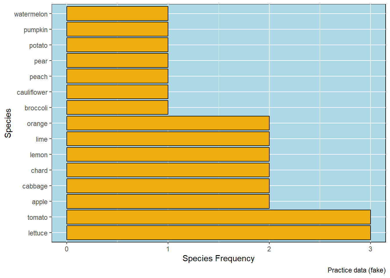
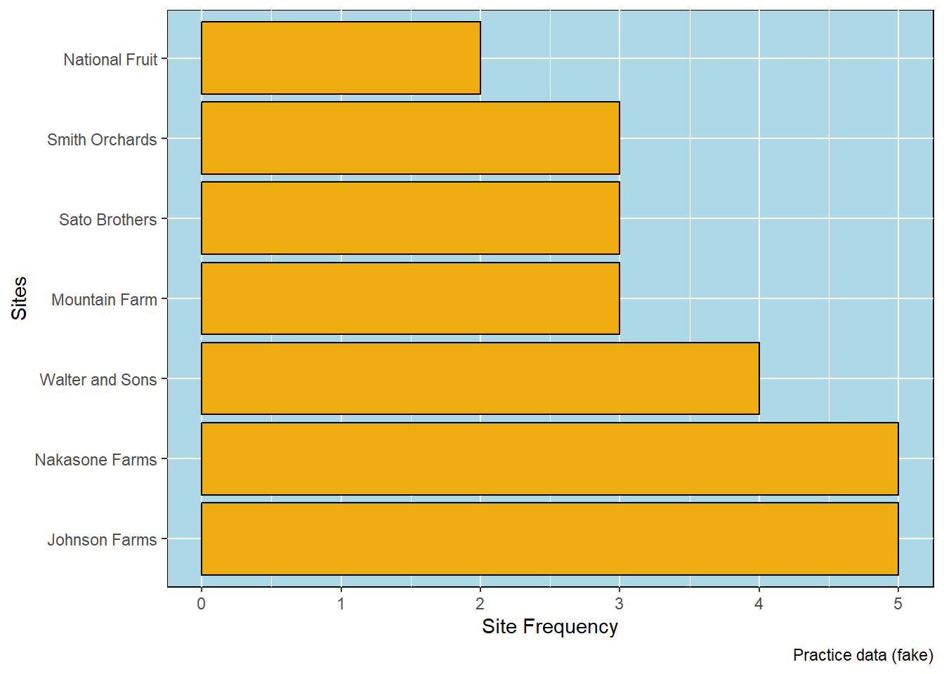
Several graphics can be created at this point. The most basic is a frequency distribution of the values for either the rows of the table (in this case, Farms) or the columns (here, Vegetables). The frequency shows the number of vegetables per farm, or the number of farms with a particular vegetable.

The first chart shows the frequency distribution of the number of vegetables grown on each farm. Note that it is possible to dig down into the statistics of the data distribution, such as the mean or median number of vegetables on each farm. But that goes beyond the basic data scanning that’s more useful at this stage.

## Generate a species frequency plot
plot1 <- species_freq_plot(data=data,data_source=source)

plot1

Number of farms on which each produce item was seen.

ggsave(plot=plot1, filename = "figures/04_plot1.png")

The next chart shows the number of produce items grown on each farm.

## Generate a site frequency plot
plot2 <- site_freq_plot(data=data, data_source=source)

plot2

Number of produce items seen on each farm.

ggsave(plot=plot2, filename = "figures/05_plot2.png")

2.12 Show the Two-way Table

A two-way table is a basic data organizational structure. An important characteristic is that these tables are sparsely populated. There are many cells in which there is no value (here, represented by the number zero). As a result of this characteristic, many numerical operations can’t be run (“too many missing values”). Instead, analyses are done column-wise or row-wise.

## Reformat the data to a two-way table
data_2way <- data_to_2way(data=data)

## Print table verification
data_table4 <- gt(data_2way) |>
  opt_row_striping() |>
  cols_label(Species  = "produce")  |>
  tab_source_note(
    source_note = source)  |>
  gt_add_divider(columns = "Species", 
                  style = "solid",
                  color = "gray88")

data_table4

Vegetables seen on each farm.

produce	Johnson Farms	Sato Brothers	Mountain Farm	Smith Orchards	Walter and Sons	National Fruit	Nakasone Farms
apple	0	0	1	0	0	0	1
broccoli	1	0	0	0	0	0	0
cabbage	1	0	0	0	1	0	0
cauliflower	0	0	0	0	1	0	0
chard	1	0	0	0	0	0	1
lemon	0	0	0	1	0	1	0
lettuce	1	0	0	0	1	0	1
lime	0	0	0	1	0	0	1
orange	0	0	0	1	0	1	0
peach	0	0	1	0	0	0	0
pear	0	0	1	0	0	0	0
potato	0	1	0	0	0	0	0
pumpkin	0	1	0	0	0	0	0
tomato	1	0	0	0	1	0	1
watermelon	0	1	0	0	0	0	0
Practice data (fake)

gtsave(data=data_table4, filename = "figures/06_data_table4.png")

2.13 Add Scientific Names

Identifying produce with scientific names reduces the possibility of misunderstanding due to the different names used for the same species (or varieties).

Here, we get Claude 3 to give us the scientific name and authorship for each of the produce items. Then we’ll verify the data by checking the validity of these names (when possible).

## Submit the fourth query for processing.
query <- paste(request4, "###", Spp_list, " ###")
data_rows <- claudeR(prompt = list(list(role = "user", 
                                       content = query)), 
                    model = "claude-3-opus-20240229", 
                    max_tokens = 500,
                    api_key = claude_key)

sci_names <- read_csv(file = data_rows)

## Process results from previous chunk.
answer$scientific <-
  paste0("*",answer$scientific,"* ", answer$author)

match_list <- answer |>
  dplyr::rename(authority = wfo_name) |>
  select(scientific, authority) |>
  arrange(scientific)

spp_table <- gt(match_list) |>
  fmt_markdown() |>
  opt_row_striping() |>
  tab_caption(caption = "Scientific Name Check") |>   
  tab_style(
    cell_text(v_align="top"),
    locations = cells_body()) |>
  tab_source_note(
    source_note = source) |>
  tab_footnote(
    footnote = "WFO approved name",
    locations = cells_column_labels(columns=authority))

## Show the table.
spp_table

Verification of the species.

scientific	authority1
Beta vulgaris subsp. vulgaris (L.) Schübl. & G. Martens, 1834	NA
Brassica oleracea var. botrytis L., 1753	NA
Brassica oleracea var. capitata L., 1753	NA
Brassica oleracea var. italica Plenck, 1794	NA
Citrullus lanatus (Thunb.) Matsum. & Nakai, 1916	NA
Citrus aurantiifolia (Christm.) Swingle, 1913	NA
Citrus limon (L.) Osbeck, 1765	NA
Citrus sinensis (L.) Osbeck, 1765	NA
Cucurbita pepo L., 1753	NA
Lactuca sativa L., 1753	NA
Malus domestica Borkh., 1803	NA
Prunus persica (L.) Batsch, 1801	NA
Pyrus communis L., 1753	NA
Solanum lycopersicum L., 1753	NA
Solanum tuberosum L., 1753	NA
Practice data (fake)
1 WFO approved name

## Save the table.
gtsave(spp_table,filename = "figures/07_data_table5.png")

2.14 Make the Species Table Multilingual

Some of the farmers might not use the English common names for the produce. Claude 3 can do the translation for us.

## Make the scientific names into a list. 
name_list <- list(sci_names$scientific)  

## Submit the fifth query for processing. 
query <- paste(request5, "###", name_list, " ###") 
data_rows <- claudeR(prompt = list(list(role = "user",      
                     content = query)),                      
                     model = "claude-3-opus-20240229",                            max_tokens = 1000,
                     api_key = claude_key)  

## Read the result. 
spanish_names <- read_csv(file = data_rows)  

## Put the Spanish names with the previous names. 
merged_names <- merge.data.frame(sci_names,
                                 spanish_names, 
                                 all.x = TRUE)   

## Get the names fixed up. 
merged_names <- merged_names |>   
  dplyr::rename(market = common) |>   
  mutate(scientific = paste0("*",scientific,"*")) |>   
  select(scientific, market, spanish) 

## Create the multilingual table. 
data_table5 <- gt(merged_names) |>
  fmt_markdown() |>   
  tab_caption(caption = "Multilingual Table") |>   
  tab_footnote(footnote = "Translated by Claude 3",     
               locations = cells_column_labels(columns=spanish)) |>    
  tab_source_note(source_note = paste0("Source: ",source)) |>
  tab_options(table.align = "left")

## Show the table. 
data_table5  

Multilingual Table

scientific	market	spanish1
Beta vulgaris subsp. vulgaris	chard	Betabel
Brassica oleracea var. botrytis	cauliflower	Coliflor
Brassica oleracea var. capitata	cabbage	Col
Brassica oleracea var. italica	broccoli	Brócoli
Citrullus lanatus	watermelon	Sandía
Citrus aurantiifolia	lime	Lima
Citrus limon	lemon	Limón
Citrus sinensis	orange	Naranja
Cucurbita pepo	pumpkin	Calabaza
Lactuca sativa	lettuce	Lechuga
Malus domestica	apple	Manzana
Prunus persica	peach	Durazno
Pyrus communis	pear	Pera
Solanum lycopersicum	tomato	Jitomate
Solanum tuberosum	potato	Papa
Source: Practice data (fake)
1 Translated by Claude 3

## Save the table. 
gtsave(data=data_table5, filename = "figures/08_data_table6.png")

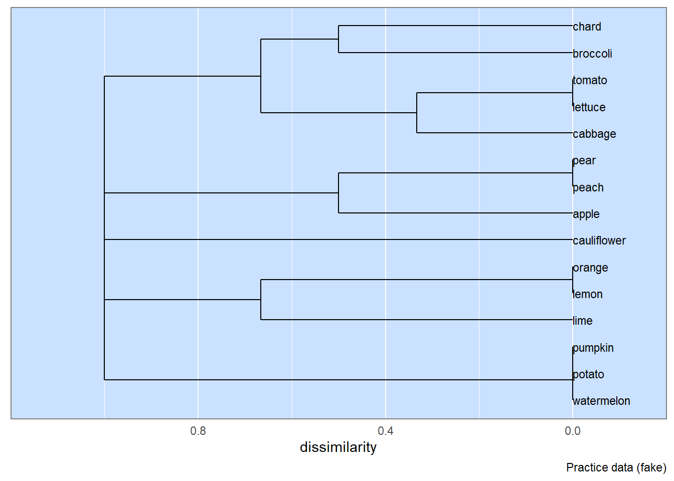
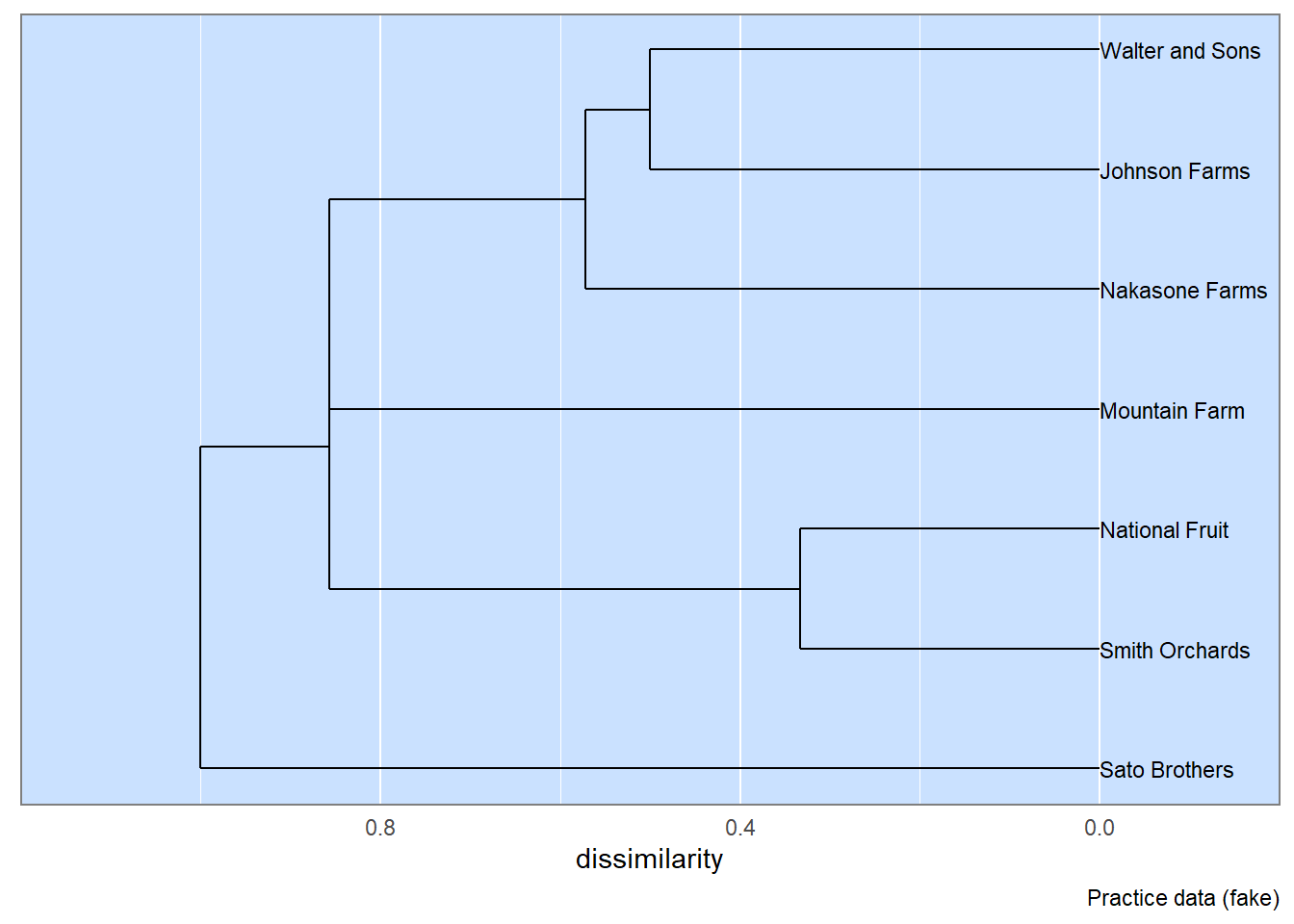
2.15 Build Dendrogram Visualizations

Two-way table are subjected to similarity analyses and the resulting similarity matrix is visualized with a dendrogram. There are two basic visualizations: species (from a row-wise analysis) and sites (from a column-wise analysis).

## Work-around (temporary).
data_source <- source

## Create the dendrogram.
plot3 <- species_dendrogram(data_2way=data_2way)

plot3

ggsave(plot=plot3, filename = "figures/09_plot3.png")

## Create the dendrogram.
plot4 <- site_dendrogram(data_2way=data_2way)

plot4

ggsave(plot=plot4, filename = "figures/10_plot4.png")

2.16 Map the Farm Locations

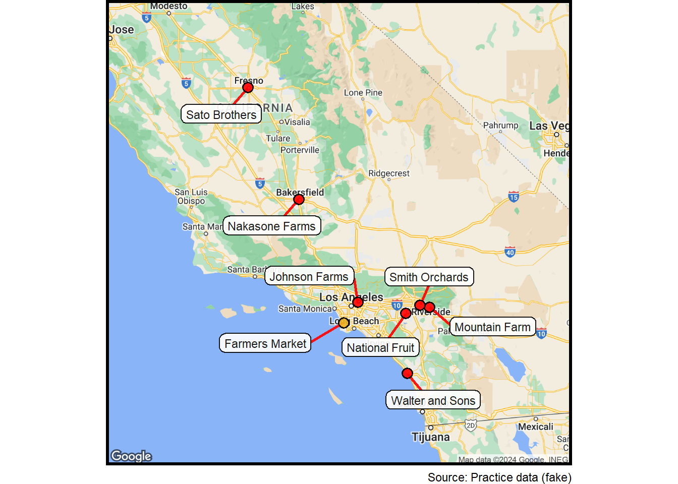
Earlier, we used Claude 3 to obtain the locations of the farms from the city that was posted on the farm-stand banner. These city data were collected as part of the dialog captured during the reconnaissance. Here we map these data.

## Reconfigure the data to add point colors
all_locs <- data2
all_locs$point_color <- "red"
all_locs <- dplyr::select(all_locs,text,lat,lon,point_color)
target_loc <- data3
target_loc$point_color <- "goldenrod2"
all_locs <- rbind(target_loc, all_locs)

## Expand the map to make sure all locations are included.
column$margin <- 0.4

## Generate a basemap.
basemap <- site_google_basemap(datatable = all_locs)

## Make smaller labels.
column$label_text_size <- 3.0

## Generate a map.
location_map <- ggmap(basemap) +
  site_labels(datatable = all_locs) +
  site_points(datatable = all_locs) +
  simple_black_box +
  labs(caption = paste0("Source: ",source))

location_map

ggsave(plot=location_map, filename = "figures/11_location_map.png")

2.17 Add Elevations to the Location Data

We can use the site (i.e., farm) locations to retrieve elevation data. This is done with the Google Maps API.

## Get the elevations (meters) from Google Maps.
## Uses the stored Google Maps API key.
elev <- google_elevation(df_locations = data2, 
                         location_type = "individual",
                         key=google_key())

## Add elevations to the location data.
data2 <- cbind(data2,elev$results$elevation)

## Convert elevations to Imperial units.
data2 <- data2 |>
  dplyr::rename(elevation_m = "elev$results$elevation") |>
  mutate(elev_ft = elevation_m * 3.28084) |>
  mutate(elev_ft = round(elev_ft,digits=0)) |>
  select(-elevation_m)

## Make a new table of the location data.
data_table6 <- gt(data2) |>
  tab_caption(caption = data3$text) |>
  cols_label(text    = "location")  |>
  cols_label(elev_ft = "elevation") |>
  tab_footnote(
    footnote = "feet",
    locations = cells_column_labels(columns=elev_ft)) |> 
  tab_source_note(source_note = paste0("Source: ",source))  

data_table6

Farmers Market

location	city	lat	lon	elevation1
Johnson Farms	Alhambra	34.0952	-118.1271	489
Sato Brothers	Fresno	36.7378	-119.7871	295
Mountain Farm	Yucaipa	34.0336	-117.0430	2628
Smith Orchards	Redlands	34.0556	-117.1825	1359
Walter and Sons	Oceanside	33.1959	-117.3795	68
National Fruit	Riverside	33.9533	-117.3962	830
Nakasone Farms	Bakersfield	35.3733	-119.0187	404
Source: Practice data (fake)
1 feet

gtsave(data=data_table6, filename = "figures/12_data_table7.png")

2.18 Calculate Farm to Market Distances

We know the locations of both the market and farms. These data let us calculate the straight-line distance between these endpoints.

## The target location.
target <- c(data3$lon, data3$lat)

## Calculate each distance.
for(i in 1:nrow(data2)){
    ## Isolate each location as the origin
    origin <- c(data2$lon[i], data2$lat[i])
    dist_meters <- distm(target, origin, fun=distHaversine)
    ## Convert meter to miles
    dist_miles <- dist_meters * 0.000621371
    data2$dist_mi[i] <- round(dist_miles,digits = 0)
    } ## end for loop

## Remove the geographic coordinates and sort.
data2 <- data2 |>
  arrange(dist_mi) |>
  select(-lat, -lon)

## Create a new table
data_table7 <- gt(data2) |>
  tab_caption(caption = data3$text) |>
  cols_label(text    = "location")  |>
  cols_label(elev_ft = "elevation") |>
  cols_label(dist_mi = "distance")  |>
  tab_footnote(
    footnote = "feet",
    locations = cells_column_labels(columns=elev_ft)) |> 
  tab_footnote(
    footnote = "miles, distance to target",
    locations = cells_column_labels(columns=dist_mi)) |> 
  tab_source_note(source_note = paste0("Source: ",source))  

data_table7

Farmers Market

location	city	elevation1	distance2
Johnson Farms	Alhambra	489	22
National Fruit	Riverside	830	55
Smith Orchards	Redlands	1359	68
Walter and Sons	Oceanside	68	71
Mountain Farm	Yucaipa	2628	76
Nakasone Farms	Bakersfield	404	113
Sato Brothers	Fresno	295	217
Source: Practice data (fake)
1 feet
2 miles, distance to target

gtsave(data=data_table7, filename = "figures/13_data_table8.png")

## Calculate summary statistics
dist_stats <- summary(data2$dist_mi)

## Make a summary table.
loc <- NULL
loc[1] <- "Closest"
loc[2] <- "Farthest"
loc[3] <- "Average"

miles    <- NULL
miles[1] <- dist_stats[1]
miles[2] <- dist_stats[6]
miles[3] <- dist_stats[3]

dist_summary <- data.frame(loc,miles)

gt(dist_summary)|>
  tab_header(title = "Farm to Market Distances") |>
  cols_label(loc = "farm")  |>
  tab_source_note(source_note = paste0("Source: ",source))  

Farm to Market Distances
farm	miles
Closest	22
Farthest	217
Average	71
Source: Practice data (fake)