A map is a very useful addition to understanding the day’s activities. Grouping is going to be used to show the locations of the photos. Without grouping, there would be too many points (and labels). The overlap of information would be too confusing.
The mapping will use the Sitemap package (described in another of the Quarto docs). This requires the activation of the Google Maps API key.
3.1 Setup the Libraries and Data
The code here uses two APIs: OpenAI and Google Maps.
Show the code
## Standard Packageslibrary(tidyverse) ## Lots of useful stufflibrary(gt) ## Make Tableslibrary(ggplot2) ## Create chartslibrary(devtools) ## Load packages from GitHub## Specialized librarieslibrary(httr) ## Send requests and receive responseslibrary(jsonlite) ## Handle the request formattinglibrary(pdftools) ## Handle PDF fileslibrary(base64enc) ## Convert image files to base64 encodinglibrary(googledrive) ## Download Google Doc fileslibrary(curl) ## The force behind the httr functionslibrary(ggmap) ## Google (and other) map functions## Get the accessOAI package (do this just once)## install_github("kimbridges/accessOAI")## install_github("kimbridges/sitemaps")## Initialize the kimbridges librarieslibrary(accessOAI)library(sitemaps)## Initialize some things that rarely change.LLM <-"gpt-4o"LLM_alt <-"gpt-3.5-turbo"## (text only)temp <-1apiKey <-Sys.getenv("OPENAI_API_KEY")My_Key <-Sys.getenv("GGMAP_GOOGLE_API_KEY")## Register the Google Maps API Key.register_google(key = My_Key, account_type ="standard")## Use two functions from sitemaps to initialize columneterscolumn <-site_styles()hide <-site_google_hides()## Establish a theme that improves the appearance of a map.## this theme removes the axis labels and ## puts a border around the map. No legend.simple_black_box <-theme_void() +theme(panel.border =element_rect(color ="black", fill=NA, linewidth=2),legend.position ="none")## Get Baseinfo (originates in photos chapter)baseinfo <-read.table("baseinfo.txt")source <- baseinfo$sourcefolder <- baseinfo$folderthumbs_folder <- baseinfo$thumbs_folderfiles_folder <- baseinfo$files_folder
3.2 Read the Location File
The image locations come from a temporary file created in a previous section.
Show the code
## Get the locations.file_location <-paste0(files_folder,"/photo_info.txt")data <-read.table(file = file_location)n_rows <-nrow(data)
3.3 Group with Distances & Time Intervals
The grouping will be done with an OpenAI request. The basic data are the distances between successive photos, along with the time interval between the images.
There isn’t any information provided about the size of the distance or time interval to be used for the grouping. That’s something decided by the LLM. Note that this may change if this is run multiple times.
Show the code
## OpenAI Prompts.role <-"You know how to make groups of photos based on the time the photo was taken, the time since the previous photo, and the distance between successive photos. Your goal is to group the photos so that a map can be drawn with all the photos using group locations rather than individual photo locations. You know that a group can consist of from one to several photos. You know how travel days are structured with meals, activities and events and you know how to aggregate similar things documented by the photos. You do not make up activities or events that are not part of the set of photos."prompt <-"You are an expert at inferring daily activities of a person traveling from a log of their photos. The log has information for each photo including the photo number, the location at which the photo was taken (lat, lon), the distance (in meters) moved from the previous photo location, the time (in minutes) between this and the previous photo, and the photo caption. Assign a group ID called 'group' to each photo. Create a CSV table with the photo number and group ID, lat, and lon. Respond with just the CSV table and no comments."## Do the analysis. response <-analyzeTXT(analysis_text = data,AI_role = role,analysis_prompt = prompt,LLM = LLM,apiKey = apiKey,connecttimeout =90)## Check the response. ## cat(response)## Strip some unnecessary data from the response.clean_string <-substr(response,8,9999)## Read the data.group_data <-read_csv(file = clean_string)group_data <- group_data[1:nrow(data),]group <- group_data[,2]## Add the group to the data table.data <-cbind(data,group)## Save the data, just in case.file_location <-paste0(files_folder,"/photo_info.txt")write.table(data, file = file_location)
3.4 Process Groups for Mapping
Photo that are nearby each other need to have the photo labels consolidated. This eliminates crowding.
Show the code
## Get the data from the temp file.file_location <-paste0(files_folder,"/photo_info.txt")data <-read.table(file = file_location)## Add a photo number (= row number).data$number <-as.integer(data$number)## Group and use the groups to get the stats.data_grouped <- data |>group_by(group) |>mutate(mean_lat =mean(lat)) |>mutate(mean_lon =mean(lon)) |>mutate(start =min(number)) |>mutate(end =max(number))## Save just the first row of each group.data_map <- data_grouped |>group_by(group) |>filter(row_number()==1) |>rename(text = number)## Create the label text (first and last in the set).for (i in1:nrow(data_map)){if (data_map$start[i] == data_map$end[i]) { data_map$text[i] <- data_map$start[i] } else { data_map$text[i] <-paste0(data_map$start[i],"-", data_map$end[i]) } } ## end for loop## Simplify the dataset and adjust the names (for Sitemaps).data_map <- data_map |>select(group, text, mean_lat, mean_lon) |>rename(lat = mean_lat, lon = mean_lon)
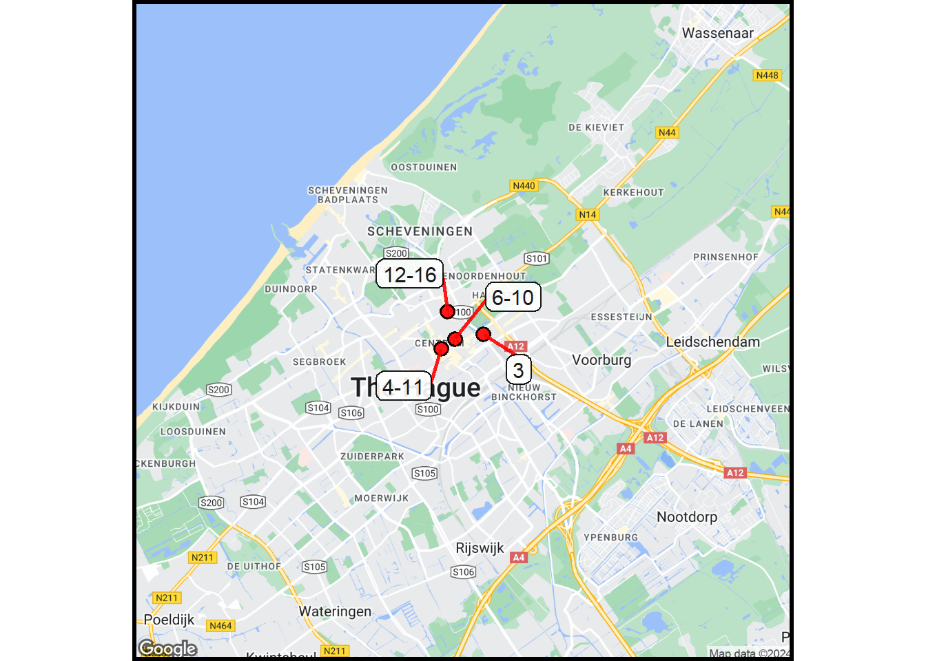
3.5 Make the Map
This is going to use the Sitemaps functions. These routines take a structured data frame (columns have specific names) and produce a map with points with labels.
There are a few photo locations, specifically 1-3, that are far from where the other photos were taken. This is a problem of scale, and it is a problem. This scale-related situation is solved here by filtering out the distant points. The remaining points are mapped.
It would be possible to fix this problem by doing groupings (as shown in the previous chunk) at two different scales. Not doing this is a recognized shortcoming here and solving it is beyond the scope of this rapid prototype.
Show the code
## HERE IS THE GROUPING WORK-AROUND## Filter to get area with most photos.data_map2 <- data_map |>filter(group >2)## Create the basemap.column$margin <-3basemap <-site_google_basemap(datatable = data_map2,styles = column)## Plot the map.ggmap(basemap) +site_points(datatable = data_map2) +site_labels(datatable = data_map2) + simple_black_box