5  International Borders

This section has a few example of country plots from different regions of the world. This shows that with the "world" parameter, the map_data function works for most of the world’s countries.

5.1 Initialize the Libraries and Data

There are a few things needed to setup the environment.

## Set an option for the read_csv function
options(readr.show_col_types = FALSE) ## Suppress warning msg

## Initialize the Standard Libraries
library(readr)
library(ggplot2)
library(dplyr)
library(gt)

## Initialize sitemaps & plain_maps
##devtools::install_github("kimbridges/sitemaps")
library(sitemaps)
##devtools::install_github("kimbridges/plainmaps")
library(plainmaps)

## Map Libraries
library(mapdata)
library(sf)

## Initialize defaults for Sitemaps
column <- site_styles()
hide   <- site_google_hides()

## Themes
plain_background_theme <- theme(
  panel.border     = element_blank(), 
  panel.grid       = element_blank(),
  panel.background = element_blank(),
  axis.text        = element_blank(),
  axis.ticks       = element_blank(),
  axis.title       = element_blank()) 

island_map_theme <- theme(
  panel.border = element_rect(color     = "black", 
                              fill      = NA, 
                              linewidth = 0.7),   
  panel.grid     = element_blank(),
  panel.background = element_rect(fill = "lightsteelblue1"),
  axis.text      = element_blank(), 
  axis.ticks     = element_blank(), 
  axis.title     = element_blank())

5.2 A Useful Function: region_plot

Much of the time, you’re likely to want a basic outline of a country. The following function lets you create this outline quite simply. Its use is demonstrated in the plots of several countries.

The function extracts the country border(s) and does the plotting. If multiple countries are extracted (as in the following example), the plot handles the fill and border color the same for all the countries.

This function plots one or more countries using a single color. There are some default values that can be changed for specific uses:

• fill: a single color used to fill the area inside the border.

• color: the color for the border outline.

• lineweight: the thickness of the border line.

• coord: a value to control the aspect ratio. A value of 1.3 (default) works best for mid-latitude countries. For countries near the equator, reduce the value (e.g., 1.0). This might take some visual adjustment so the aspect ratio of the country looks familiar.

• mytheme: the name of a theme to control the map appearance.

You don’t need to use this function. It is straightforward to adapt the code to extract a single country. Here, it’s convenient and avoids too much code repetition.

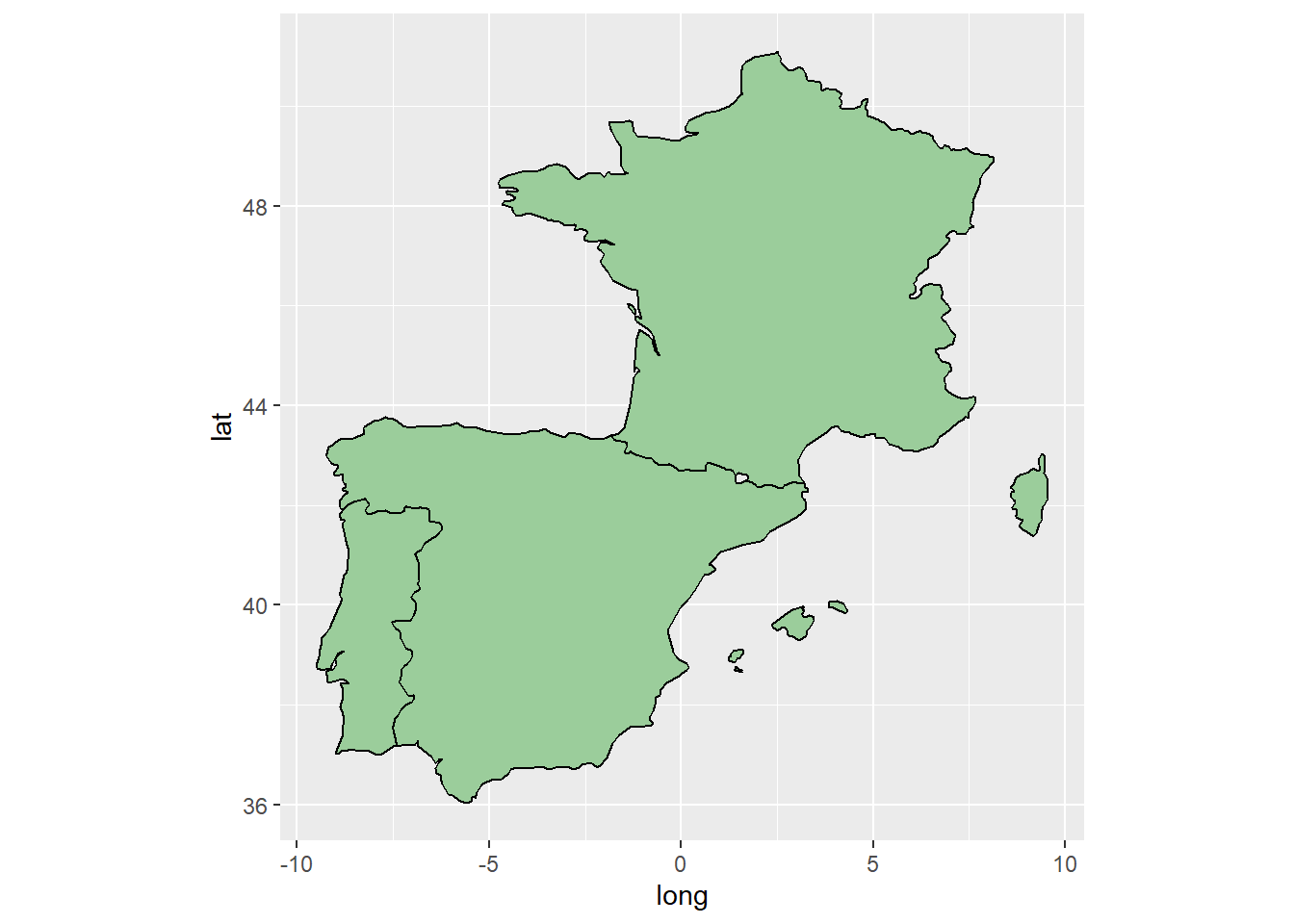
5.3 Extract Several Countries

This example uses the default version of the region_plot function.

Three adjacent countries are extracted and plotted.

## Extract the three countries
three <- map_data("world", region =c("Portugal",
                                    "Spain",
                                    "France"))

## Generate the plot using the region_plot function
region_plot(region = three)

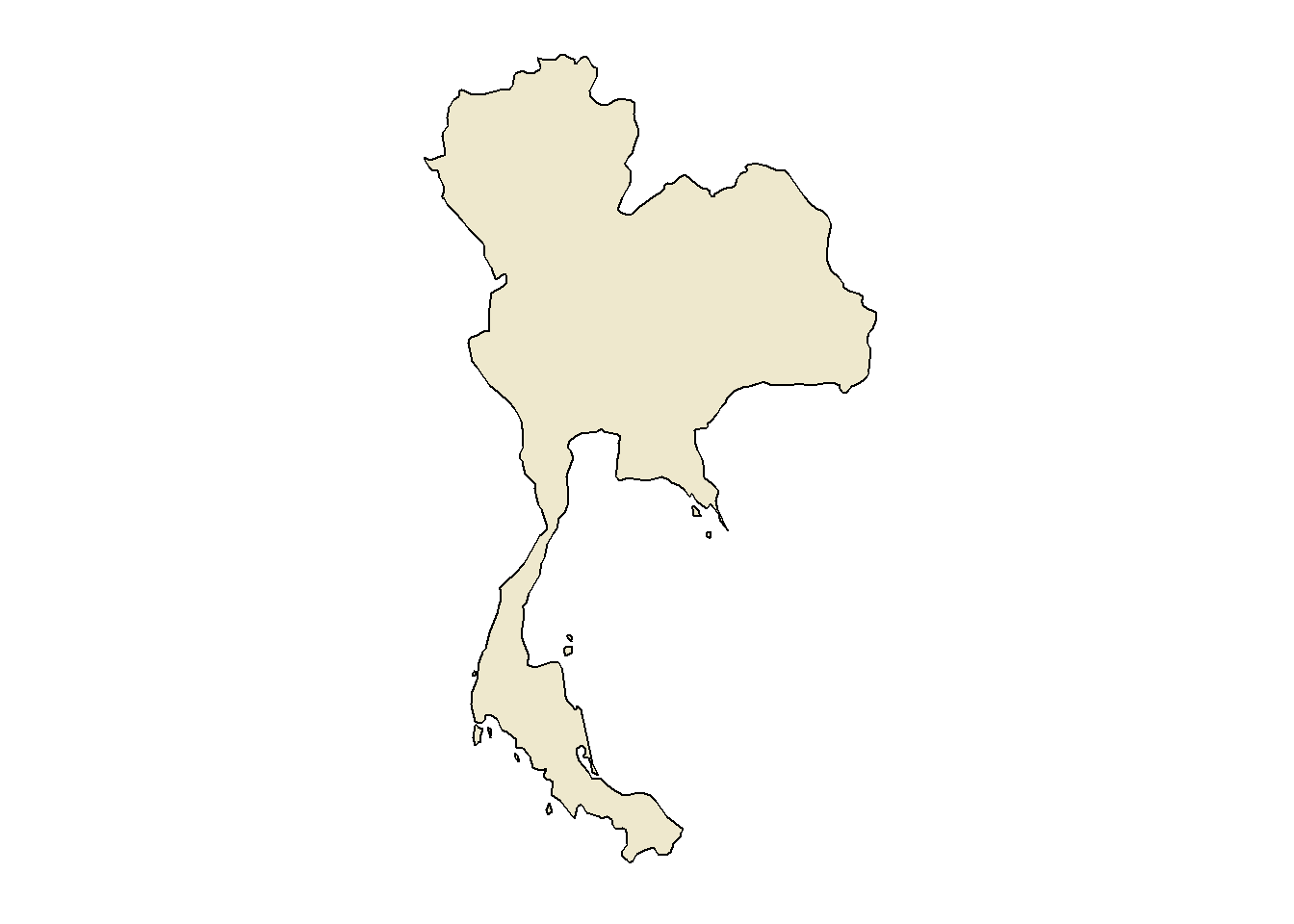
5.4 Add a Theme

Here, there are several parameter changes to the region_plot function shown in this example. In particular, note the change to the aspect ratio, coord, as this country is close to the Equator.

A theme was defined in the Initialization section called the “plain_background_theme”. Using this theme removes all the information outside the country borders.

## Extract the Thailand border.
thailand <- map_data("world", region = "Thailand")

## Generate the plot using the region_plot function.
thailand_map <- region_plot(region  = thailand, 
                            coord   = 1.0, 
                            fill    = "cornsilk2",
                            mytheme = plain_background_theme)

## Show the map.
thailand_map 

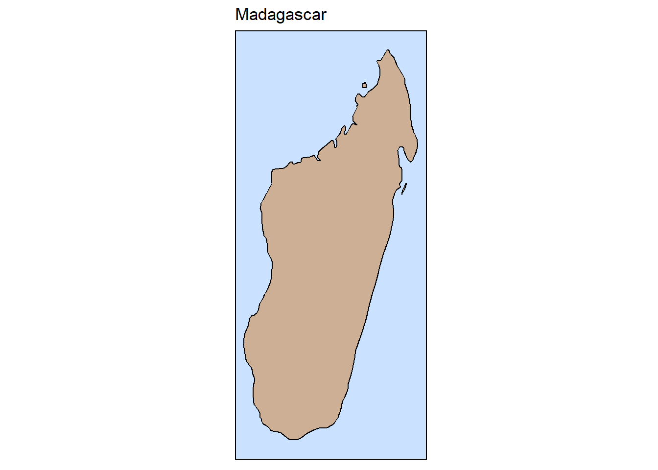
5.5 Modify More Parameters

This example has a few changes to the region_plot defaults and an addition to the plot.

• fill: the color is changed to "peachpuff3".

• labs: gives a title to the map.

• coord: adjusts the aspect ratio (lat/lon ratio).

## Specify the country
country <- "Madagascar"

## Extract the Madagascar border.
mad <- map_data("world", region = country)

## Generate the plot using the region_plot function.
mad_map <- region_plot(region = mad,
                       fill = "peachpuff3",
                       coord = 1.2,
                       mytheme = island_map_theme) +
           ## Label the axes   
           labs(title = country) 

## Show the map using an island theme.
mad_map

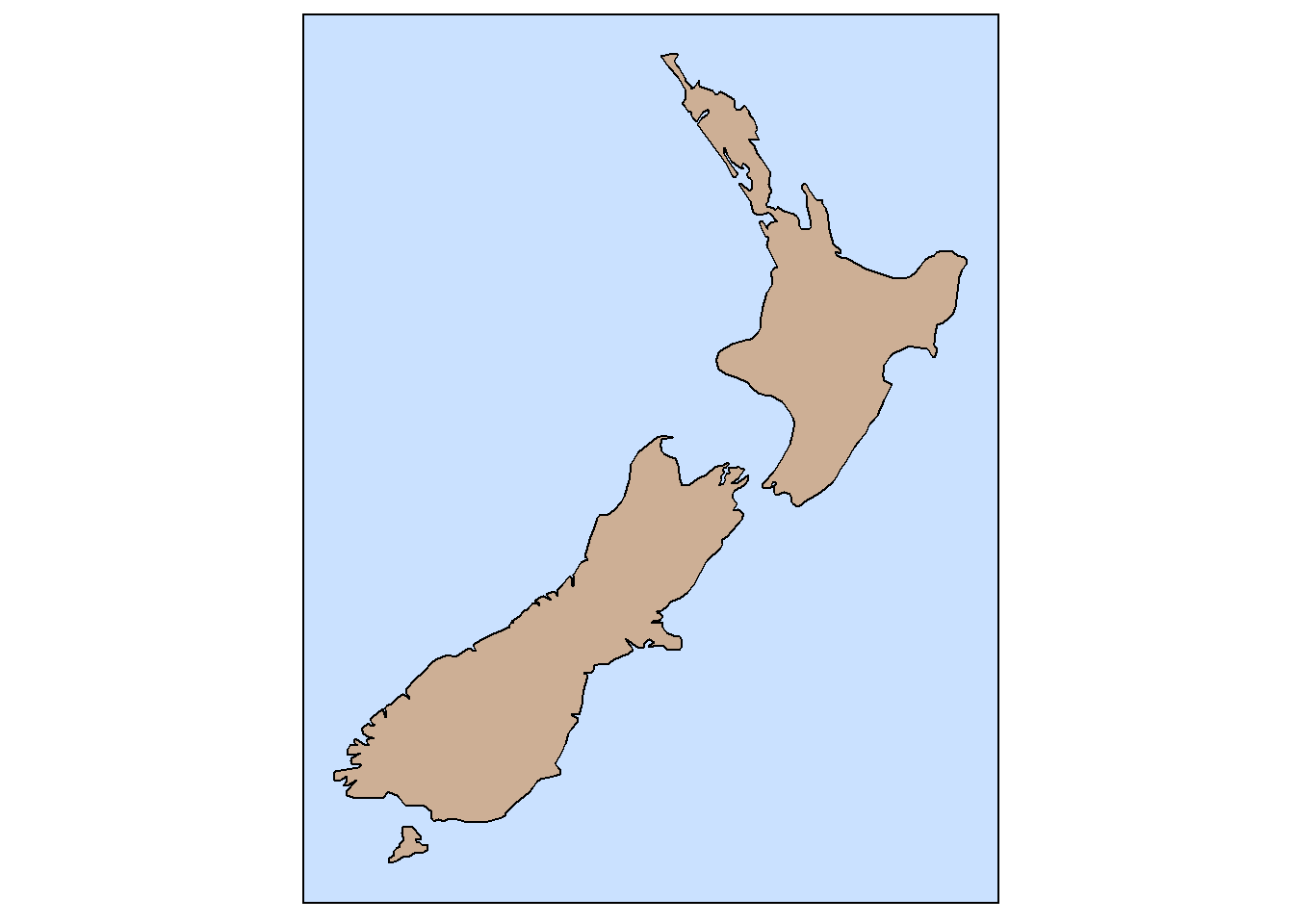
5.6 Clean-up Problems

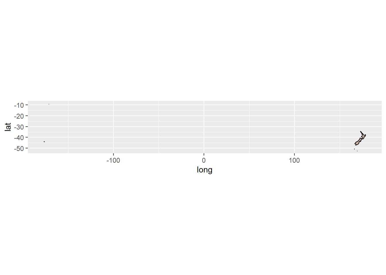
Sometimes, the data for a map produces unusual and unacceptable results.

Here is an example. We’ll extract and plot New Zealand.

## Extract the New Zealand border.
NZ <- map_data("world", region = "New Zealand")

## Generate the plot using the region_plot function.
NZ_map <- region_plot(region = NZ,
                       fill = "peachpuff3",
                       coord = 1.2)
## Plot the map.
NZ_map

Yike! There are some places that are far away from the main islands in New Zealand. We can get rid of these tiny places for our purposes.

Filtering out places that aren’t needed uses the dplyr filter function.

Here’s how.

Examine the extracted map data. In this example, it is the NZ variable. Examine this variable’s values by opening it (click on the name in the Enviroment list). You’ll see a column with names of the places that make up the country. Note the value of the group variable for each place you want to retain. For NZ, three places are selected (9 = South Island, 11 = North Island, 3 = Stewart Island). Use these three values to do the filtering.

## Do the filtering.
NZ_filter <- NZ |>
  dplyr::filter(group == 9 | group == 11 | group == 3)

## Create a map with the filtered data.
NZ_filter_map <- region_plot(region = NZ_filter,
                       fill = "peachpuff3",
                       coord = 1.2,
                       mytheme = island_map_theme)

## Show the map.
NZ_filter_map