Placing a reference overlay on a map is a very common requirement. Adding an overlay is similar to doing a cut-out as seen in several of the other chapter. The procedure is more general, in a way, as reference overlays may have a complex geometry, not just a rectangular shape.
This chapter shows a few techniques for creating a general overlay. Note that there are a few situations where you can use existing geographic information (e.g., counties within US States) where the process is more like specialized choropleth mapping (see the Choropleth chapter for details).
7.1 Initialize the Libraries and Data
There is some code that reads a locally-stored file of boundary data. These data were stored in the Shapefiles chapter. Here they are read so they can be used in several chunks in this chapter.
Show the code
## Set an option for the read_csv functionoptions(readr.show_col_types =FALSE) ## Suppress warning msg## Initialize the Standard Librarieslibrary(readr)library(ggplot2)library(dplyr)library(gt)## Install the sitemaps & plainmaps packages (uncomment; run once)## library(devtools)## install_github("kimbridges/sitemaps")## install_github("kimbridges/plainmaps")## Sitemapslibrary(sitemaps)library(plainmaps)## Map Librarieslibrary(mapdata)library(sf)## Special Librarieslibrary(geosphere) ## Calculate distances between points## Initialize defaults for Sitemapscolumn <-site_styles()hide <-site_google_hides()## Read stored border dataoahu_border_400 <-read_csv(col_names =TRUE, show_col_types =FALSE,file ="hawaii_400/oahu_outline.csv")oahu_border_200 <-read_csv(col_names =TRUE, show_col_types =FALSE,file ="hawaii_200/oahu_outline.csv")hawaii_border_400 <-read_csv(col_names =TRUE, show_col_types =FALSE,file ="hawaii_400/hawaii_outline.csv")## Themesplain_background_theme <-theme(panel.border =element_blank(), panel.grid =element_blank(),panel.background =element_blank(),axis.text =element_blank(),axis.ticks =element_blank(),axis.title =element_blank()) island_map_theme <-theme(panel.border =element_rect(color ="black", fill =NA, linewidth =0.7), panel.grid =element_blank(),panel.background =element_rect(fill ="lightsteelblue1"),axis.text =element_blank(), axis.ticks =element_blank(), axis.title =element_blank())
7.2 Functions
Several functions are introduced here. The purpose is to assist in the creation and use of overlays that are drawn on top of the plain maps.
corner2poly: This function converts a data frame with just two diagonal corners into a five-row polygon. The names of the columns in both the corner and five-row polygon are the same: “lon” and “lat”.
kml_polygon: Converts an outline from Google Earth Pro (in kml format) to geographic coordinates (lat, lon).
complete_outline: Put a snipped section of a basemap boundary (such as a coastline) together with a partial overlay boundary to create an overlay that exactly overlays the basemap boundary. This function uses an internal function (find_closest) to locate the boundary section to be snipped.
7.3 Creating an Overlay Polygon
If you are creating your own overlay polygons, there is an important requirement.
Overlay polygons are closed outlines. That is, the first and last data rows must have the same coordinate values.
Rectangles: A rectangular overlay will have five data rows, one for each corner and the last one closing the polygon.
The corner2poly function can be used, when necessary, to simplify the creation of the rectangle with five data rows.
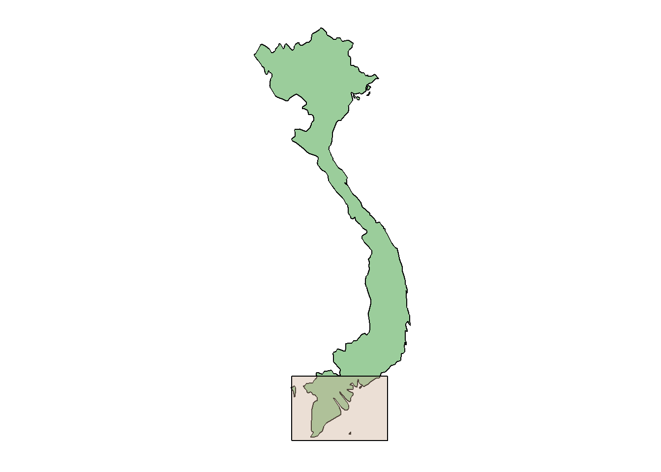
This shape overlay is likely useful when the detailed boundaries are not known or they are too detailed to be useful. The placement of an overlay rectangle can imply just a general area.
Here is an example.
Show the code
## Get the corners of the overlay rectangle.two_corner <-read_csv(col_names=TRUE,file="lon, lat 103.89350, 8.45876 108.38352, 10.77965")rect <-corner2poly(corners = two_corner)## Get the basemap.VN <-map_data("world", region ="Vietnam")## Create the basemap.VN_map <-region_plot(region = VN)## Plot the basemap with the overlayVN_map + plain_background_theme +geom_polygon(data=rect,aes(x = lon, y = lat,group =1), fill ="peachpuff3", color ="black",alpha =0.4)
If you are combining a country map with a detailed map that shows data locations, you’ll want to use the bounding box created with the sitemaps functions. See the Sitemaps chapter for more information and examples.
7.4 Creating Polygon Overlays
Sometimes, you need to create an overlay that’s more complex than a rectangle. For example, your overlay might outline the area of a national park or the area occupied by a village. The goal is to input the overlay corners (called vertices) without having to type the geographic coordinates.
7.4.1 Google Earth Pro
Google Earth Pro is a free utility. It is very useful as it provides detailed satellite views of the entire planet. This software also has some useful tools.
Google Earth Pro has a function (Add Polygon) that lets you click on polygon vertices (corner points) to create a polygon that holds the geographic coordinates. A function is available (kml_polygon) that will extract the coordinates into a data frame that can be used with ggplot.
This process is quite straightforward if there are recognizable landmarks on the Google Earth map. That’s shown in the first example. Later, an overlay is added to Google Earth so that there is guidance on where to place the vertices.
Note that if you are creating several overlays, you should do each one separately. They are combined when you create the map in ggplot.
7.4.2 Recognizable Vertices
The procedure starts by opening Google Earth Pro. Here are the steps.
Search or navigate with the map controls to the location where you will create the overlay.
Click on the menu Add tab and click on Polygon.
The pop-up box has several tabs at the top. Choose the Style, Color tab.
Go to the Area section and change the value for Opacity to something like 50%. As you create the polygon it will be filled. You want to see through the fill color. The opacity lets you do this.
DO NOT CLICK OK.
Hover over the map. The cursor will be a square box with small lines crossing each side. Center the box on a vertex and click. Move to the next point and click. You’ll see a line. Another click and you get a triangle.
Keep clicking on points until you’ve completed the polygon.
NOW YOU SHOULD CLICK OK.
7.4.2.1 Saving the polygon
You’ll see an entry called “Untitled Polygon” over in the Places listing (likely at the left side of the screen) .
Right click on this entry and choose “Save Place As…”. A regular “Save file” menu box will appear. Navigate to the proper folder.
Choose an appropriate File name for the polygon.
Be sure to change the Save as type to “Kml” (the default is Kmz which is a zipped version of the Kml file).
7.4.2.2 Correcting Polygon Errors
You can edit the polygon points after you’ve clicked OK to end the polygon creation process.
Right click on the “Untitled Polygon” entry in the Places listing. Choose “Properties”.
The big menu box will pop up with Google Earth - Edit Polygon on the header at the top. You’ll probably need to move this box out of the way if it is covering your polygon.
Modifying point locations: Note the very tiny red dots at each vertex. If you click on one of these, it will change color to green. Then you can click and drag the point to a new location.
Deleting points: If you need to delete a point, choose it (turns green) and press the delete key.
Adding points: Add a point by clicking on a line between two points.
When you are done editing the polygon, click the OK button on the big menu box.
You might need to save your polygon again.
Show the code
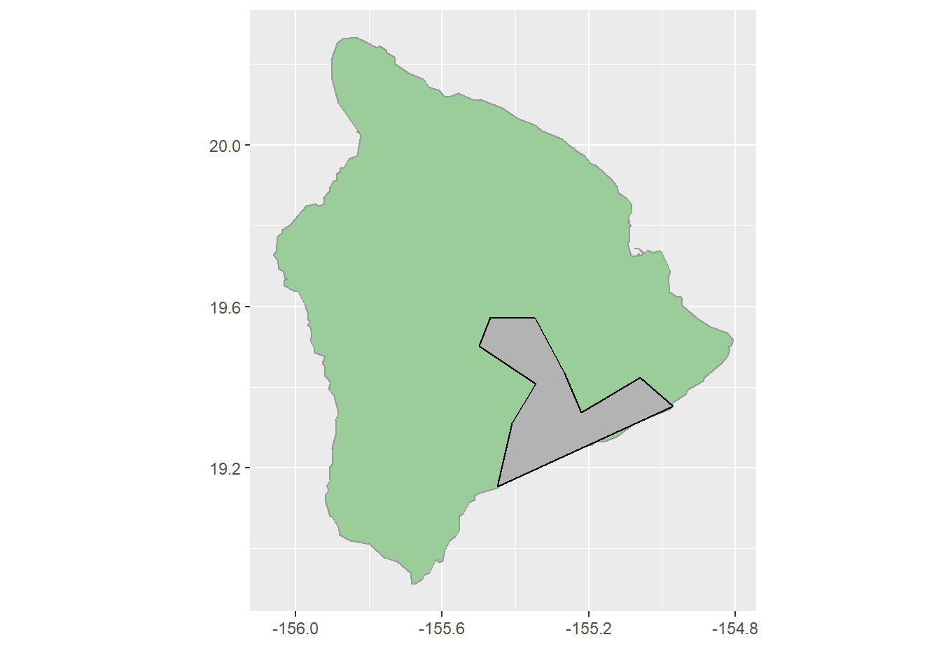
## kml data are stored in an external (local) folder.kml_data <-"overlays/hvnp_rough_draft.kml"## Convert from KML to coordinates (lat,lon).overlay_coord <-kml_polygon(overlay_kml = kml_data)
Reading layer `hvnp_rough_draft.kml' from data source
  `P:\Emerging\plain_maps\overlays\hvnp_rough_draft.kml' using driver `KML'
Simple feature collection with 1 feature and 2 fields
Geometry type: POLYGON
Dimension:     XYZ
Bounding box:  xmin: -155.4997 ymin: 19.15205 xmax: -154.9704 ymax: 19.57277
z_range:       zmin: 0 zmax: 0
Geodetic CRS:  WGS 84
Show the code
## Plot the overlay on top of the basemap.ggplot() +## Basemapgeom_polygon(data=hawaii_border_400, aes(x=lon,y=lat), fill="darkseagreen3", color ="gray60") +## Overlaygeom_polygon(data=overlay_coord, aes(x=lon,y=lat),fill="gray70", color ="black") +## Suppress the axis nameslabs(x="",y="") +## Adjust coordinatescoord_fixed(1.1)
Note that the overlay doesn’t follow the coastline very well. That’s intentional here as this is a rough designation of an area. It is possible to use the coastline as part of the overlay. The way to do it is shown in an example shown below.
7.5 Trace an Overlay
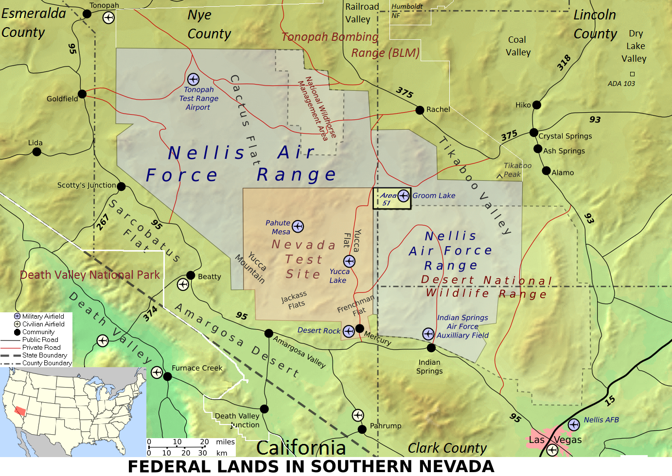
Sometimes, a reference map isn’t set up to allow you to capture the geographic coordinates of a place you want to use as an overlay. Here is an example map showing the location of the Nevada Test Site, the location of hundreds of atomic tests.
You can use this map as an overlay in Google Earth Pro.
Navigate in Google Earth Pro to the approximate location of the overlay and make the scale so that you will see the entire overlay when it is added.
Use the Add Image Overlay button to get a popup menu. Then fill in the Name for the overlay and Browse to get the file for the Link.
The overlay will have green lines at the corners, a green bar with a diamond, and a green plus at the center. Click and drag the plus to move the overlay. Click or Shift-Click the corners to scale the overlay (Shift-Click keeps the aspect ratio). Click and drag the diamond to rotate the overlay.
It helps to pick some reference points that are common to the overlay and the Google Earth Pro map. Use the transparency slider to look back and forth between the overlay and the basemap.
Once the overlay is aligned, click OK on the popup menu. That “freezes” the location of the overlay.
Now you can use the Add Polygon button to create the vertices of your overlay boundary. Save this set of boundary points as a KML file in a convenient directory.
The overlay_kml function reads the KML file and converts the KML code to geographic coordinates.
Show the code
## Get a basemap for Nevada.## Extract the set of US states.states <-map_data("state")## Remove just one state (Nevada) from the set.NV <- states %>%filter(region =="nevada")## Specify the location of the KML overlay.kml_data <-"overlays/nevada_test_site.kml"## Use the KML location to retrieve and convert the data.nts <-kml_polygon(overlay_kml = kml_data)
Reading layer `nevada_test_site.kml' from data source
  `P:\Emerging\plain_maps\overlays\nevada_test_site.kml' using driver `KML'
Simple feature collection with 1 feature and 2 fields
Geometry type: POLYGON
Dimension:     XYZ
Bounding box:  xmin: -116.5119 ymin: 36.60521 xmax: -115.849 ymax: 37.22034
z_range:       zmin: 0 zmax: 0
Geodetic CRS:  WGS 84
Show the code
## Plot the map and overlay.ggplot(NV) +## Basemapgeom_polygon(aes(x = long, y = lat,group = group), fill ="peachpuff3", color ="black") +## Overlaygeom_polygon(data=nts, aes(x=lon,y=lat),fill="gray70", color ="black") +## Suppress the axis nameslabs(x="",y="") +## Adjust coordinatescoord_fixed(1.1)
7.6 Use a Country Border in an Overlay
Borders are often quite detailed. You really don’t want to retrace a border section when an overlay includes a border. Instead, it’s best just to clip out a section of the border and include the geographic vertices in the overlay outline.
A border extraction function has been written to simplify this process. Basically, you create the set of vertex coordinates for the overlay outline except for the border section. The function complete_outline uses the partial overlay and the border outline. The two are combined to form a complete overlay outline.
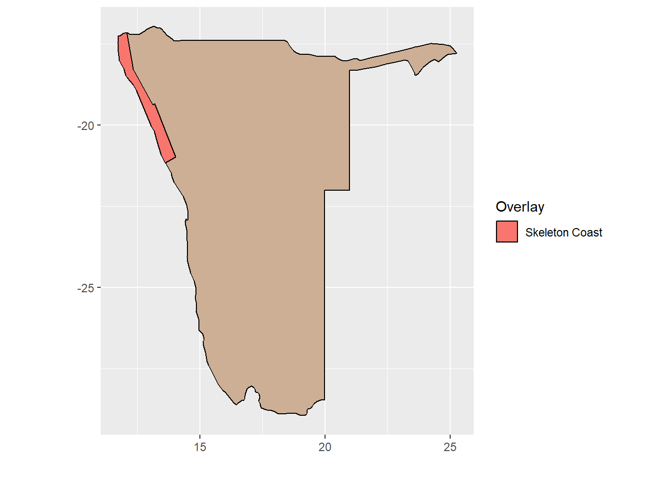
This is shown in the next chunk. Note that the inland area of the skeleton coast is the partial outline. The complete_outline function finds the points on the coast that are closest to the ends of the partial outline and automatically extracts the coastal segment and adds this to the overlay.
Show the code
## Get coordinate outline for the country.namibia_border <-map_data("world", region ="Namibia")## Rename the longitude column (lon) and save just the coordinates.namibia <- namibia_border |> dplyr::rename(lon = long) |>select(lat,lon)## Create a partial overlay (missing the part along the border).## Outline points digitized manually from south to north.skeleton_coast <-read_csv(file ="lat, lon -21.16724, 13.60947 -20.97544, 14.01753 -19.34054, 13.18062 -19.37062, 13.11675 -18.27945, 12.33405 -17.14559, 12.06748 -17.18604, 11.91856 -17.25693, 11.79078 -17.23646, 11.74826")## Combine the partial overlay with the section of border.skeleton_overlay <-complete_outline(border = namibia,overlay = skeleton_coast)## Create a plain map of the region.namibia_map <-region_plot(region = namibia_border,fill ="peachpuff3") ## Put the overlay on top of the plain map & do the legend.namibia_map +## Add the overlaygeom_polygon(data=skeleton_overlay,aes(x=lon,y=lat,group=1,fill="lightsalmon1"),color="black") +## Add a legendscale_fill_discrete(name ="Overlay",labels ="Skeleton Coast") +## Suppress the axis nameslabs(x="",y="")