Shapefiles are a special format used to store geographic data. They are very commonly used, especially with GIS applications. As a result, borders for many areas are available for download from Internet sites.
The shapefiles used in the examples were downloaded to a local folder. To recreate the examples, get the shapefiles from the cited source and store them on your computer.
6.1 Building Hawaii Maps From Shapefiles
There are no maps for Hawaii available with the map_data function. There also don’t seem to be any border files with lat,lon geographic coordinates.
It’s a lot of work to digitize the outlines for the islands. Instead, we can extract and convert island outline from a shapefile so they can be used in the various map plotting functions.
The source of the Hawaiian Islands shapefile is a website made available by the State of Hawai`i. This is a high resolution file. The detail exceeds our needs here.
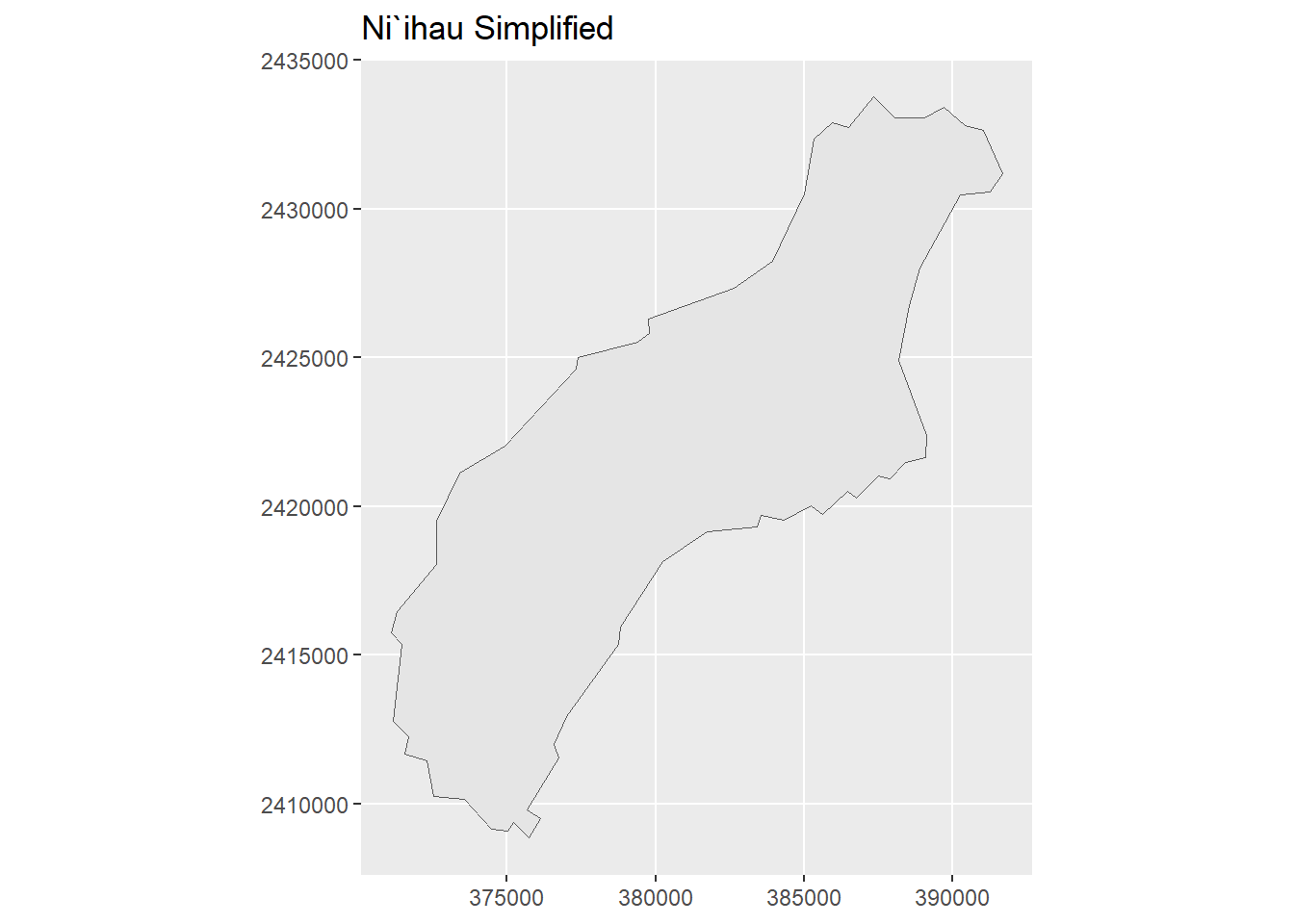
The processing shown in the next chunk retrieves the shapefiles from a locally-stored copy. The coordinates are converted from UTM values to more customary lat,lon coordinate data. After this, the coordinates are simplified so the island boundary details are more consistent with the general plotting needs.
One file is created for each of the major islands.
The island files, in the lat,lon coordinate format, are stored in a local folder for use in other chapters (and other projects). Note that in practice, it is useful to store versions of each area (in this case, islands) at different resolutions.
6.2 Data Source
This chapter uses some shape files to get the outlines of the islands in the state of Hawai`i. These shape files are available at this website:
There are a few things needed to setup the environment.
Show the code
## Set an option for the read_csv functionoptions(readr.show_col_types =FALSE) ## Suppress warning msg## Initialize the Standard Librarieslibrary(readr)library(ggplot2)library(dplyr)library(gt)## Sitemapslibrary(sitemaps)library(plainmaps)## Map Librarieslibrary(mapdata)library(sf)library(oce) ## Tool used for coordinate conversion## Themesplain_background_theme <-theme(panel.border =element_blank(), panel.grid =element_blank(),panel.background =element_blank(),axis.text =element_blank(),axis.ticks =element_blank(),axis.title =element_blank()) island_map_theme <-theme(panel.border =element_rect(color ="black", fill =NA, linewidth =0.7), panel.grid =element_blank(),panel.background =element_rect(fill ="lightsteelblue1"),axis.text =element_blank(), axis.ticks =element_blank(), axis.title =element_blank())## Initialize defaults for Sitemapscolumn <-site_styles()hide <-site_google_hides()
6.4 Reading the Data
The shapefiles were downloaded as a zip file and unzipped to a local folder named “540”. Inside the 540 folder, Island_boundaries.shp is the key file. You know this as it is the only file with the “.shp” type.
Referencing the “.shp” file provides enough information that the data extraction function (st_read) brings in information from the other files in the folder.
There is a coordinate transformation step that takes the NAD83 UTM (Zone 4 North) coordinates and puts the projection on the WGS84 ellipsoid using the Spherical Mercator projection.
The boundary data are still bundled with other information, such as the grouping of borders when there are multiple boundaries (e.g., small islands surrounding a main island). (Later, you’ll see the group parameter being used to gather these multiple borders into one set.)
Show the code
## Read shapefile from local storage##hawaii_file <- "540/Island_boundaries.shp"hawaii_file <-"hawaii_coastlines/coast_n83.shp"hawaii_shape <-st_read(hawaii_file)
Reading layer `coast_n83' from data source
  `P:\Emerging\plain_maps\hawaii_coastlines\coast_n83.shp' using driver `ESRI Shapefile'
Simple feature collection with 13 features and 5 fields
Geometry type: POLYGON
Dimension:     XY
Bounding box:  xmin: 371124.5 ymin: 2094231 xmax: 940278.9 ymax: 2458612
Projected CRS: NAD83 / UTM zone 4N
Show the code
## Transform UTM coordinates to lat,lon##coord <- st_transform(hawaii_shape, crs=4326)##head(coord, 20)
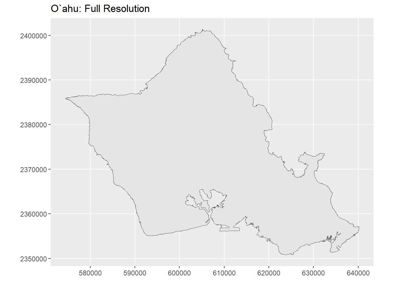
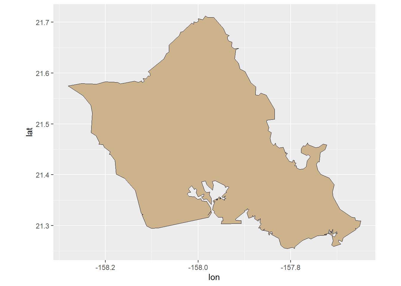
It’s a good idea to check one of the island boundaries to make sure that everything’s OK. We’ll do this by plotting O`ahu.
6.4.1 Different plotting function
The maps that aren’t built from shapefiles use the geom_polygon function in ggmaps. The shapefile data uses a similar, but slightly different function, geom_sf.
We can get our first look at a shapefile boundary map using the default settings.
Show the code
## Island Shape Files## 1 = Kauai## 2 = Lehua (off Niihau)## 3 = Niihau## 4 = Oahu## 5 = Ford Island## 8 = Molokai## 9 = Maui## 10 = Lanai## 11 = Molokini (off Maui - not used)## 12 = Kahoolawe## 13 = Hawaii Island## Show the full resolution of the border data for O`ahu.oahu_full <-st_geometry(hawaii_shape)[[4]]ggplot() +labs(title ="O`ahu: Full Resolution") +geom_sf(data=oahu_full)
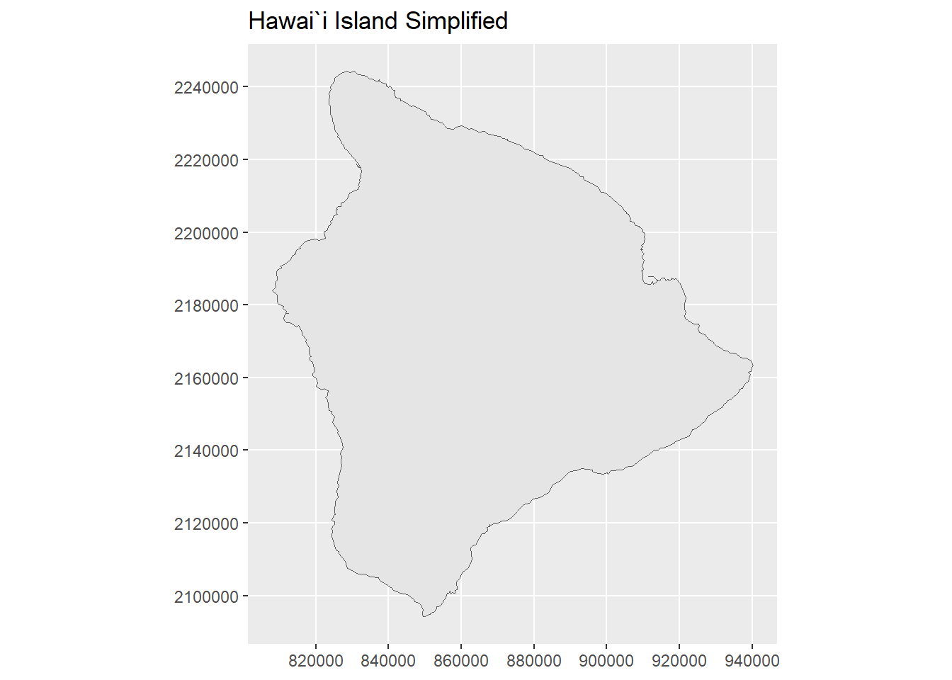
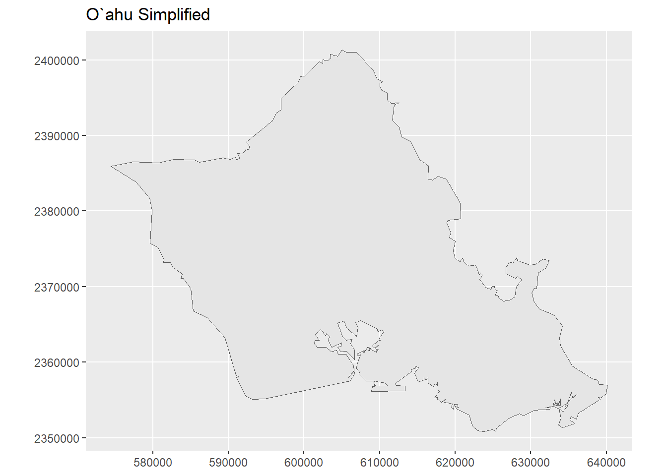
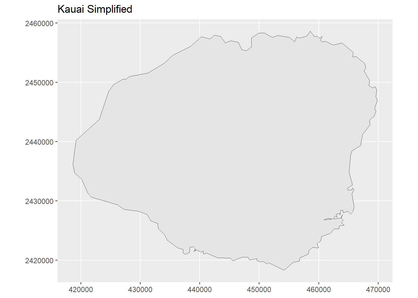
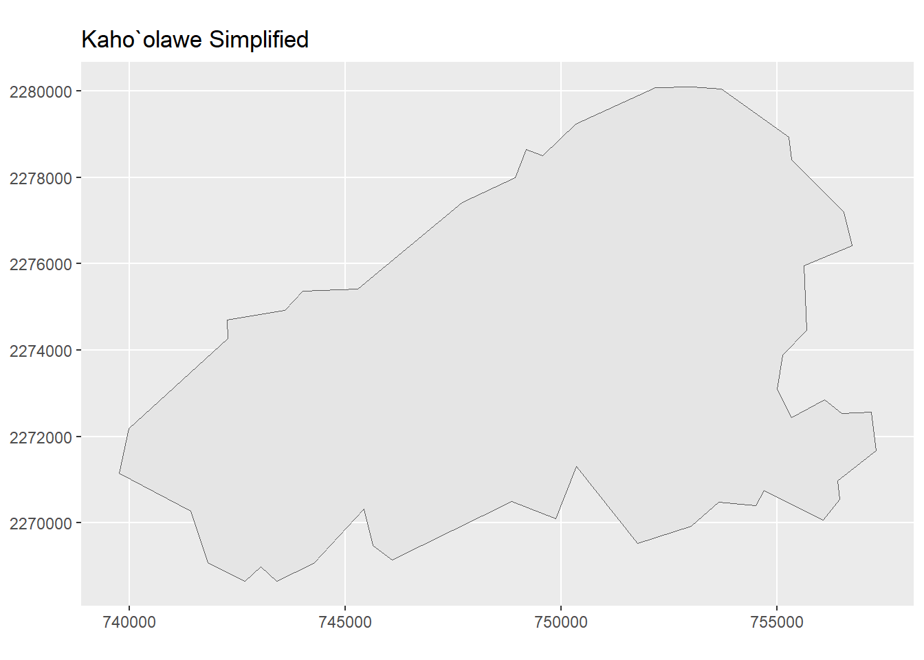
6.4.2 Simplify the border detail
While it’s nice to have high-resolution island borders, they show too much detail for our uses.
The st_simplify function reduces the details using the dTolerance parameter. The smaller the value, the more detail in the outline.
Show the code
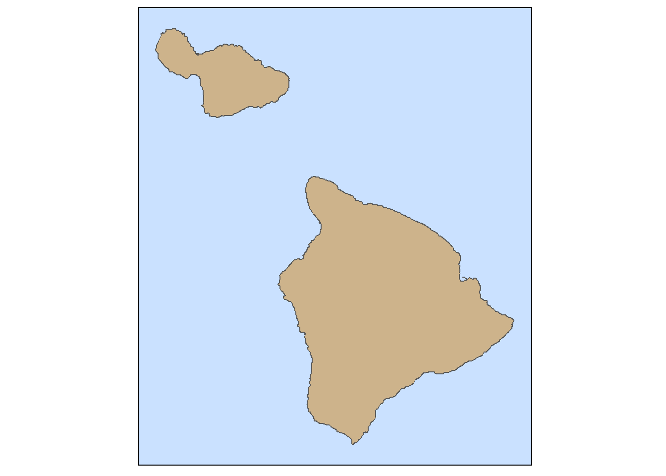
## The dTolerance value determines the simplification.dTolerance <-200## Simplify the coordinates for all the islandscoord_simple <-st_simplify(hawaii_shape, dTolerance = dTolerance)## Plot each of the islandshawaii_simple <-st_geometry(coord_simple)[[13]]ggplot() +labs(title ="Hawai`i Island Simplified") +geom_sf(data=hawaii_simple)
The island_map_theme was developed with the Hawaiian Islands in mind. However, this theme works for all area which are surrounded by water. the major feature is to have a background that shows the color of the water.
This theme also simplifies the map by removing the geographic coordinate information.
We can use this theme when we plot any island maps (e.g., Japan, Madagascar, Maui).
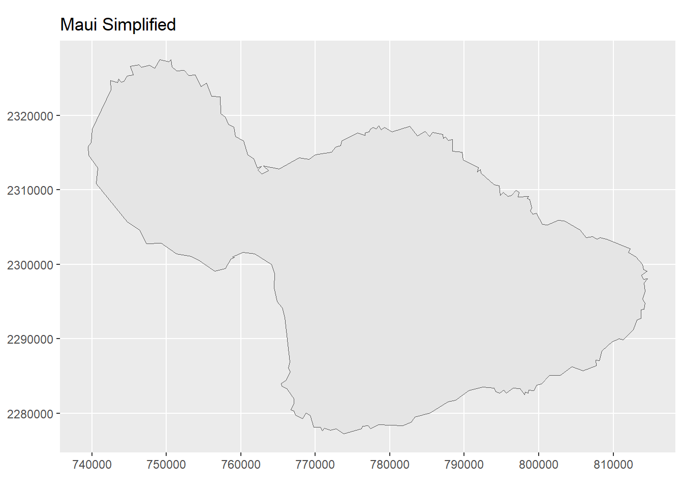
6.6 Combining Maps
A simple demonstration shows how to plot two islands together. This also uses the custom theme to simplify the background.
Show the code
## Set the linewidth for the outlines.outline_width <-0.4## Plot two islands together.ggplot() +geom_sf(data=hawaii_simple, fill="navajowhite3", linewidth=outline_width) +geom_sf(data=maui_simple, fill="navajowhite3", linewidth=outline_width) + island_map_theme
6.7 Convert UTM to lat,lon Degrees
A function is provided, UTM_convert, that converts the UTM coordinates to geographic lat, lon coordinates. This is useful as the ggplot functions (e.g., geom_polygon) use geographic coordinates. You’re also likely to use geographic coordinates when you obtain location data from Google Maps, such as when you are locating data points or placing map annotation.
This function allows for a general conversion of UTM coordinates. The parameter are:
location: the UTM coordinates zone: Default is 4, which works for Hawaii. You need to know this value. hemisphere: Default is “N”. km: Default is FALSE.
The use of the UTM_convert function is shown with the conversion of all the Hawaiian island boundaries to geographic coordinates.
Show the code
## Transform the data using the UTM_convert function## Note: Oahu has multiple polygons (only 1 is useful)niihau_coord <-UTM_convert(unlist(niihau_simple))kauai_coord <-UTM_convert(unlist(kauai_simple))oahu_coord <-UTM_convert(unlist(oahu_simple[[1]]))molokai_coord <-UTM_convert(unlist(molokai_simple))lanai_coord <-UTM_convert(unlist(lanai_simple))maui_coord <-UTM_convert(unlist(maui_simple))kahoolawe_coord <-UTM_convert(unlist(kahoolawe_simple))hawaii_coord <-UTM_convert(unlist(hawaii_simple))## Test by creating a map.ggplot(data=oahu_coord, aes(x=lon,y=lat)) +geom_polygon(fill="navajowhite3", linewidth=0.3,color="black") +coord_fixed(1.1)
Show the code
## Show some of the data, just to check.gt(head(oahu_coord))|>fmt_number(columns =c(lat,lon), decimals =5) |>tab_caption(caption ="O`ahu Coordinates (partial)") |>tab_source_note(source_note ="Source: Converted from a shape file")
O`ahu Coordinates (partial)
lon
lat
−158.10526
21.59389
−158.10335
21.59538
−158.10422
21.60008
−158.10773
21.60298
−158.07402
21.62814
−158.06873
21.63797
Source: Converted from a shape file
6.8 Save the Island Boundaries
The island boundaries are simple in format. There are just two columns (lat, lon) of data. There are, however, a lot of rows (each one a boundary point). As a result, it’s useful to store the boundaries in a folder on the local computer.
Show the code
## No need to run this every time.run <-"no"## Test if it should be run (anything other than "no").if(!run =="no"){## Write the CSV version of the files to a local drive.## Build a folder name (allows multiple outline versions).folder_name <-"temp"## Folder already exists on location drivewrite_csv(kauai_coord, file=paste0(folder_name,"/kauai_outline.csv"))write_csv(niihau_coord, file=paste0(folder_name,"/niihau_outline.csv"))write_csv(oahu_coord, file=paste0(folder_name,"/oahu_outline.csv"))write_csv(molokai_coord, file=paste0(folder_name,"/molokai_outline.csv"))write_csv(lanai_coord, file=paste0(folder_name,"/lanai_outline.csv"))write_csv(maui_coord, file=paste0(folder_name,"/maui_outline.csv"))write_csv(kahoolawe_coord, file=paste0(folder_name,"/kahoolawe_outline.csv"))write_csv(hawaii_coord, file=paste0(folder_name,"/hawaii_outline.csv"))} ## End run test
6.8.1 Read a Stored Boundary Map
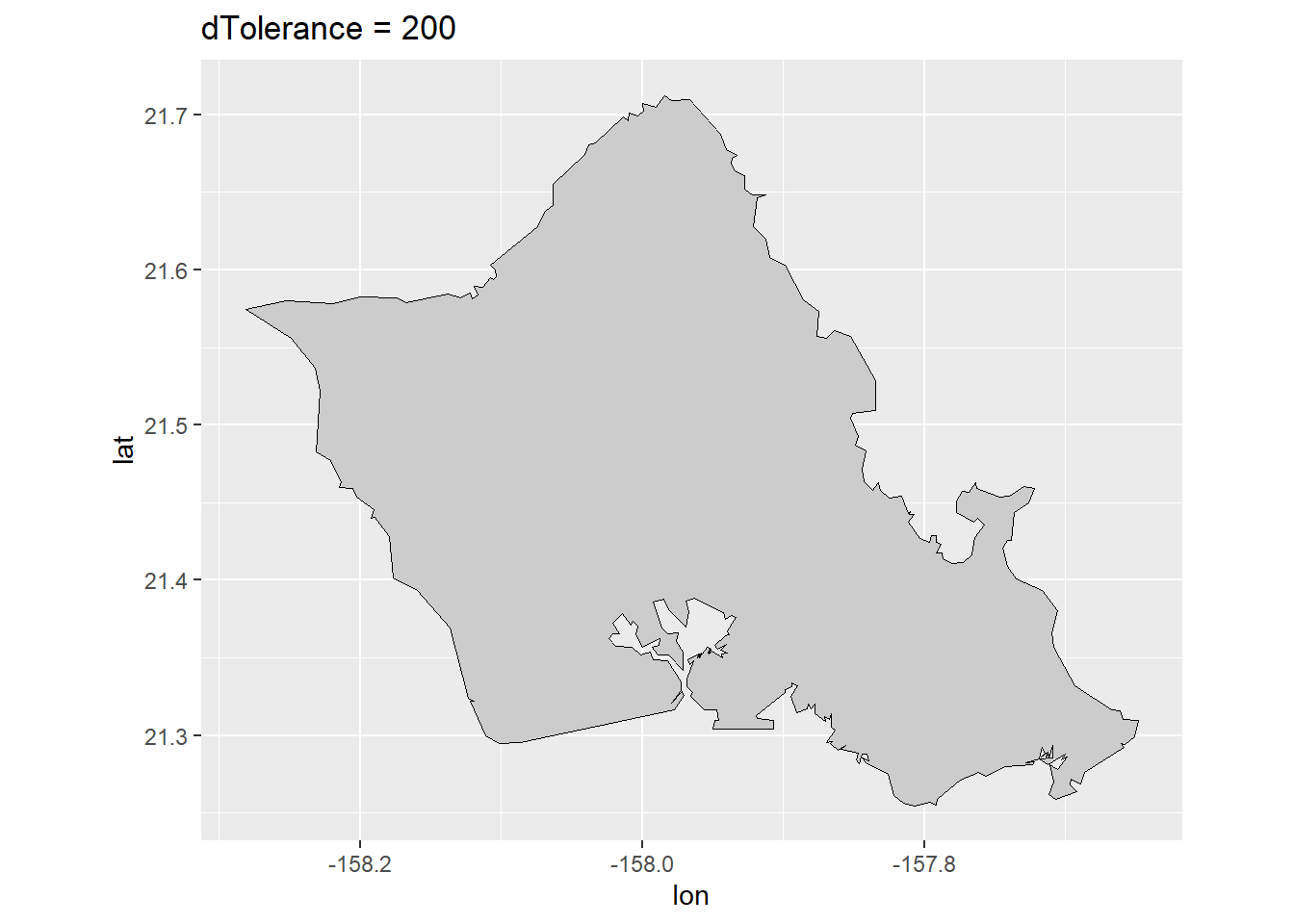
It’s a good idea to check that everything is stored OK.
Show the code
## Where are the data stored.folder_name <-"temp"## Read a stored boundary fileoahu_check <-read_csv(file=paste0(folder_name,"/oahu_outline.csv"))## Test with the mapggplot(data=oahu_check, aes(x=lon,y=lat)) +geom_polygon(fill="gray80", linewidth=0.3,color="black") +labs(title=paste0("dTolerance = ",dTolerance)) +coord_fixed(1.1)
6.9 Two Complementary Maps
Note that the island outlines are stored in the folder “inst/extdata” (not “temp”). The reason is that the “inst/extdata” folder is used in the creation of a package as a location to store data. This way, the island outlines are available for other people to use.
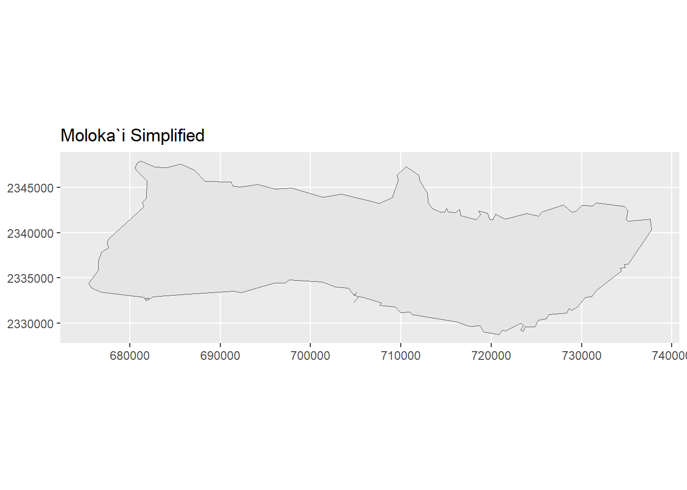
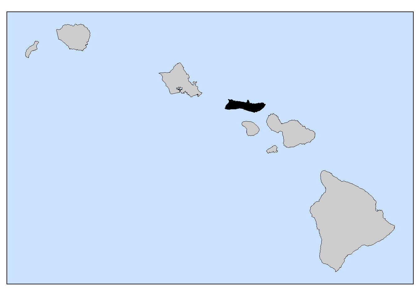
6.9.1 All Island Key Map
The map developed here has one island, Moloka’i, colored with a solid black. That’s used to identify the island in an adjacent high-resolution plot. The other islands have a neutral color.
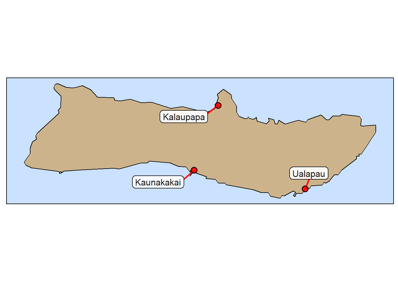
This map of a single island complements the key shown in the previous chunk. Here, the island outline shows details and locations are marked with points and labels.
Show the code
## Read the label data.data <- readr::read_csv(file ="text, lat, lon Kaunakakai, 21.08961, -157.02093 Ualapau, 21.06064, -156.83173 Kalaupapa, 21.19010, -156.98027")## Print a table of he label data.gt(data)
text
lat
lon
Kaunakakai
21.08961
-157.0209
Ualapau
21.06064
-156.8317
Kalaupapa
21.19010
-156.9803
Show the code
## Create the map with labels.ggplot() +geom_polygon(data=molokai, aes(x=lon,y=lat),fill="navajowhite3", linewidth=0.5, color="black") +site_labels(datatable = data) +site_points(datatable = data) +coord_fixed(1.1) + island_map_theme