9  Sitemap Functions

Sitemaps is a package written with functions to assist in generating basemaps (usually from Google Maps) and provide a rich set of annotations. The key feature of this package is the use of tables to specify the contents and characteristics of the annotations.

A full guide to the Sitemaps package is on this link: kim.quarto.pub/sitemaps.

We’ll just be using a bit of the sitemap functionality here.

9.1 Initialize the Libraries and Data

There are a few things needed to setup the environment.

Note the instructions (which are commented out) for installing the sitemaps package. Note that just like other R packages, once you’ve installed sitemaps on your computer, you don’t need to install it again.

A theme, called “island_map_theme”, was created specifically to plot islands surrounded by water. This theme is stored in this chunk.

There is some code that reads a locally-stored file of boundary data. These data were stored in the Shapefiles chapter. Here they are read so they can be used in several chunks in this chapter.

## Set an option for the read_csv function
options(readr.show_col_types = FALSE) ## Suppress warning msg

## Initialize the Standard Libraries
library(readr)
library(ggplot2)
library(dplyr)
library(gt)

## Install the sitemaps package (uncomment; run once)
## library(devtools)
## install_github("kimbridges/sitemaps")

## Sitemaps
library(sitemaps)
library(plainmaps)

## Map Libraries
library(mapdata)
library(sf)
library(ggmap)   ## To do geocode

## Initialize defaults for Sitemaps
column <- site_styles()
hide   <- site_google_hides()

## Themes
plain_background_theme <- theme(
  panel.border     = element_blank(), 
  panel.grid       = element_blank(),
  panel.background = element_blank(),
  axis.text        = element_blank(),
  axis.ticks       = element_blank(),
  axis.title       = element_blank()) 

island_map_theme <- theme(
  panel.border = element_rect(color     = "black", 
                              fill      = NA, 
                              linewidth = 0.7),   
  panel.grid     = element_blank(),
  panel.background = element_rect(fill = "lightsteelblue1"),
  axis.text      = element_blank(), 
  axis.ticks     = element_blank(), 
  axis.title     = element_blank())

## This theme removes the axis labels and 
## puts a border around the map. No legend.
simple_black_box <- theme_void() +
              theme(panel.border = element_rect(color = "black", 
                                   fill=NA, 
                                   size=2),
                    legend.position = "none")

## Some Hawaiian island outlines (use with read_csv).
oahu <- system.file("extdata", "oahu_outline.csv", 
                    package = "plainmaps")

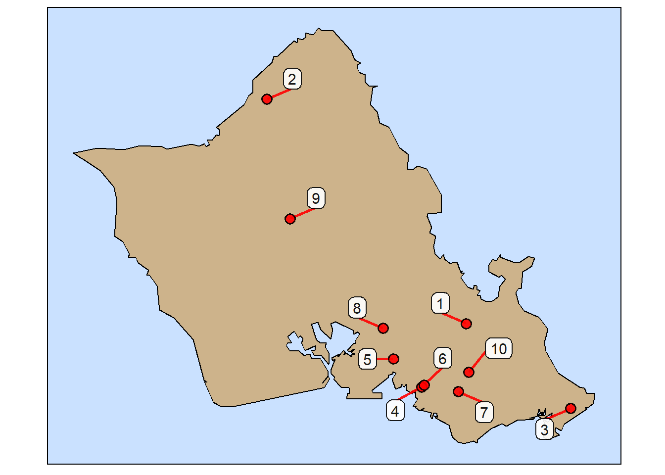
9.2 Add Points to a Hawai`i Map

The outline of the island of O`ahu was retrieved from a locally-stored file in the Initialize step (above).

The file oahu (see the Initialization section) has lat,lon data. Therefore, we can add information, via ggplot, using lat,lon location references.

The Sitemaps package has functions that simplify the addition of location information. The approach is to use data tables instead of manipulating parameters and values in the map plotting code.

The code to add the overlay information (here points and labels) is very straightforward with simple statements.

Note that the map boundaries in the following examples (which are vector objects) are not in the same format as the basemaps (which are raster objects) used in Sitemaps document examples. Therefore, plotting is done here with ggplot instead of ggmap.

The geom_point function gives us an ability to control the location and appearance of the data points. However, if there is information associated with a data point, the sitemap function site_points is easier to use. Note that the visual properties of the points are given as columns of the data table. The column names are specifically chosen to simplify the process.

## Data for the Botanical Gardens on O'ahu
data <- read_csv(file=
  "garden
    Ho'omaluhia Botanical Garden
    Waimea Valley
    Koko Crater Botanical Gardens
    Foster Botanical Garden
    Moanalua Gardens
    Lili'uokalani Botanical Garden
    Mānoa Heritage Center
    Halawa Xeriscape Garden
    Wahiawā Botanical Garden
    Lyon Arboretum")

## Prepare the data.
location <- paste0(data$garden,", Honolulu, Hawaii, USA") 

## Get the coordinates from the location.
coord <- geocode(location, output = "latlon")

## Create an ID column (call "text" to use with site_labels).
text <- c(1:nrow(data))

## Number & add the coordinates to the original data.
data <- cbind(text,data,coord)

## Show the data table.
gt(data) |> 
  fmt_number(columns = c(lat,lon), decimals = 5) |>
  tab_caption(caption = "O`ahu Botanical Gardens") |>
  tab_source_note(source_note = 
          "Source: Geocoded using Google Maps API")

O`ahu Botanical Gardens

text	garden	lon	lat
1	Ho'omaluhia Botanical Garden	−157.80455	21.38660
2	Waimea Valley	−158.04667	21.63389
3	Koko Crater Botanical Gardens	−157.67823	21.29299
4	Foster Botanical Garden	−157.85903	21.31681
5	Moanalua Gardens	−157.89305	21.34777
6	Lili'uokalani Botanical Garden	−157.85588	21.31910
7	Mānoa Heritage Center	−157.81413	21.31159
8	Halawa Xeriscape Garden	−157.90548	21.38148
9	Wahiawā Botanical Garden	−158.01808	21.50230
10	Lyon Arboretum	−157.80154	21.33297
Source: Geocoded using Google Maps API

## Get the map outline.
oahu_border <- readr::read_csv(file=oahu)

## Plot map with place locations.
ggplot() + 
  geom_polygon(data=oahu_border,
               aes(x=lon,y=lat),
               fill="navajowhite3", 
               linewidth=0.5,
               color     ="black") +
  site_labels(datatable = data) +
  site_points(datatable = data) +
  coord_fixed(1.1) +
  island_map_theme

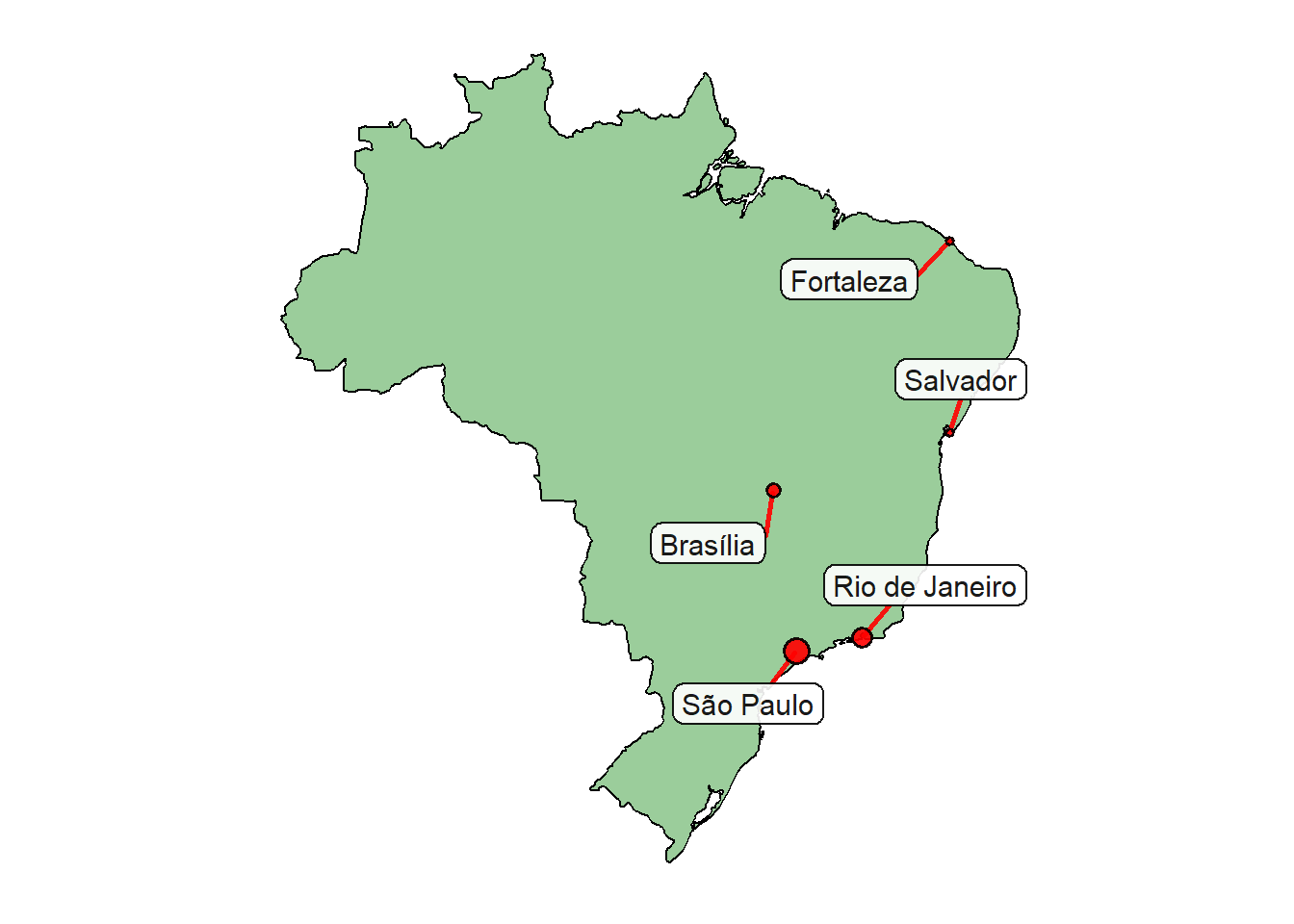
9.3 Apply Information to map_data Maps

We can use the maps extracted with map_data as basemaps and apply data points, labels and text on top using the Sitemaps functions.

There is one important addition when doing this with Sitemaps that wasn’t required when using the basic lat,lon coordinate maps such as the Hawai`i maps that were extracted from the shapefiles:

Create a column in the datatable named group with the value of 1.

Here, this datatable column was created with this statement:

cities$group <- 1

There are a few things to note in the following example:

• The column names of the datatable are changed to correspond to the names required by the Sitemaps functions (e.g., text, lat, lon).

• The population is scaled (using the site_cuts function from Sitemaps) to values which are an index based on the quartiles (i.e., 1-4). This index is placed in column named point_size so that it controls the size of the data points.

• There is a group variable used in both the creation of the basemap (the filled Brazil outline) and the datatable used for site_points and site_labels.

• The map border data uses the data labels lat and long while the sitemaps functions require the names lat and lon (note: without the “g”).

## Read city data for Brazil.
cities <- read_csv(col_names = TRUE, 
                    show_col_types = FALSE,
                    file =
    "city,           population, latitude,  longitude
     São Paulo,      12400000,   -23.5505,  -46.6333
     Rio de Janeiro,  6800000,   -22.9068,  -43.1729
     Brasília,        3100000,   -15.7942,  -47.8825
     Salvador,        2900000,   -12.9730,  -38.5023 
     Fortaleza,       2700000,    -3.7319,  -38.5267")

## Print a table to confirm the data.
gt(cities) |>
  fmt_number(
    columns  = population, 
    use_seps = TRUE,
    decimals = 0) |> 
  tab_caption(caption = "Brazil's Biggest Cities") |>
  tab_source_note(source_note="Source: Gemini AI query")

Brazil's Biggest Cities

city	population	latitude	longitude
São Paulo	12,400,000	-23.5505	-46.6333
Rio de Janeiro	6,800,000	-22.9068	-43.1729
Brasília	3,100,000	-15.7942	-47.8825
Salvador	2,900,000	-12.9730	-38.5023
Fortaleza	2,700,000	-3.7319	-38.5267
Source: Gemini AI query

## Change column names to match required names in Sitemaps.
## Note: Here it is lon (not "long").
colnames(cities)  <- c("text","population","lat","lon")

## Scale the population by quartiles for use as the point_size
cities$point_size <- site_cuts(quant_var = cities$population,
     cuttype = "quartiles4")

## Important Note: 
## You need to have a group variable in your data.
## This says which "layer" you're adding to the plot.
cities$group <- 1

## Get a Brazil border outline.
brazil <- map_data("world", region = "Brazil")

## Create a Brazil basemap (note: Here longitude is "long").
brazil_map <- ggplot(data=brazil, 
                     aes(x=long,y=lat,group=group)) +
              geom_polygon(fill      = "darkseagreen3",
                           linewidth = 0.5,
                           color     = "black")

## Show the major cities using the brazil_map.
brazil_map +
  site_labels(datatable = cities) +
  site_points(datatable = cities) +
  coord_fixed(1.1) +
  plain_background_theme

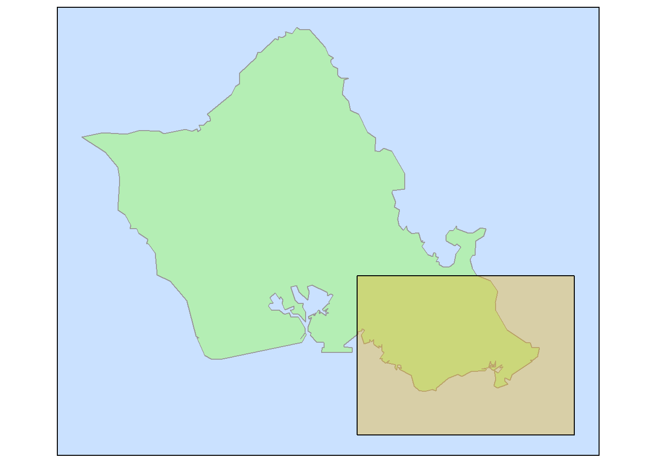
9.4 Build Maps at Two Scales

Having maps at two scales lets us use one map as a location reference for the other map.

9.4.1 Hawaii Maps: O`ahu

Two sets of boundary maps were created in the Shapefiles chapter. Files for each island were stored at two resolutions. The boundaries from the hawaii_200 folder have more detail than the maps in the hawaii_400 folder. We’ll use the more general map (loaded in the Initialization step as oahu_border_400) to show the entire island. Later, we’ll use the oahu_border_200 which has more border detail.

First, we’ll build the bit basemap map and place a bounding box on top to show the cut-out area. Then a small map is created by clipping to the limits of the bounding box.

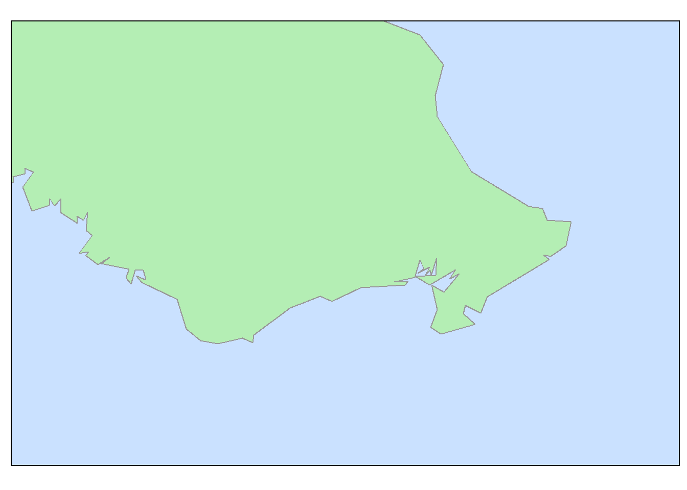
It is possible, of course, to add data to the small map.

## Create the border data. 
overview_outline <- readr::read_csv(file=
        "inst/extdata/oahu_outline.csv")

## Define the cut-out area by the corners.
range_ends <- data.frame(
  lon=c(-157.9, -157.6),
  lat=c(  21.2,   21.4))

## Make the ranges into a polygon.
box_poly <- corner2poly(range_ends)

## Create the full-sized basemap.
big_map <- ggplot() +
  ## Basemap
  geom_polygon(data=overview_outline, 
               aes(x=lon,y=lat), 
               fill="darkseagreen2", color = "gray60") +
  coord_fixed(1.1) +
  island_map_theme

## Put the range polygon on top of the basemap.
big_map_box <- big_map +
  geom_polygon(data=box_poly,
               aes(x=lon,y=lat), 
               fill="goldenrod2", 
               color = "black",
               alpha=0.4)

## Show the big reference map.
big_map_box

## Create the detail map using the cut-out ranges.
## Note: the expand=FALSE maintains the size of this area.
small_map <- big_map +
  coord_fixed(xlim=range_ends$lon, ylim=range_ends$lat,
              expand=FALSE)

## Show the cut-out map.  
small_map

9.4.2 Create the Bounding Box with Sitemaps

It is quite straightforward to create a detailed map of data locations using the sitemaps package. In particular, you don’t need to figure out the bounding box (or other basemap locating information). All the needed values are calculated using the locations of your data points.

Basemaps created using the site_google_basemap function contain not only the map data, but also some other useful information such as the bounding box coordinates. We can use this bounding box with a reference map to show the location of the basemap that has the data locations.

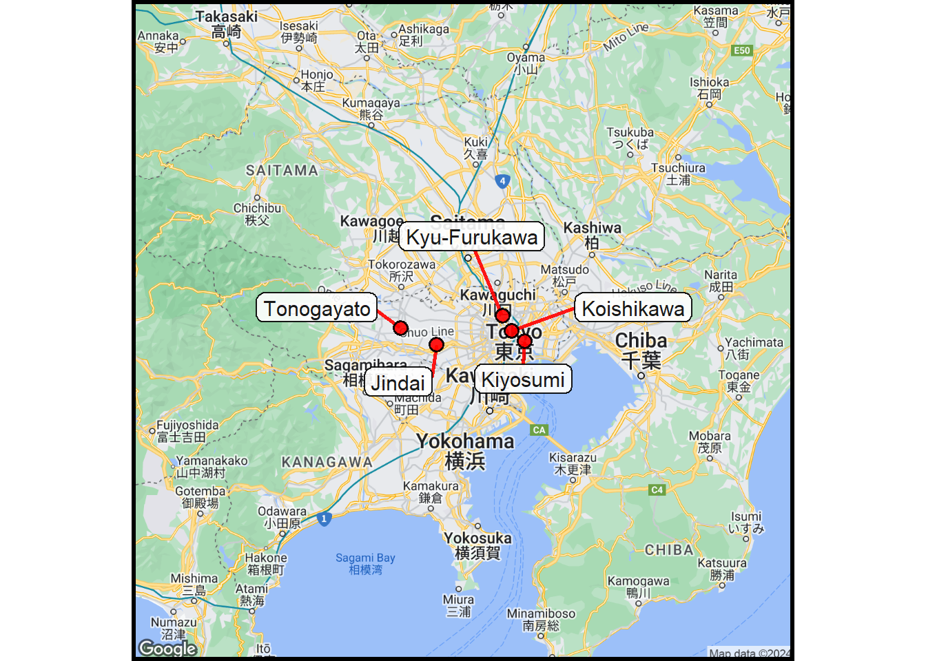
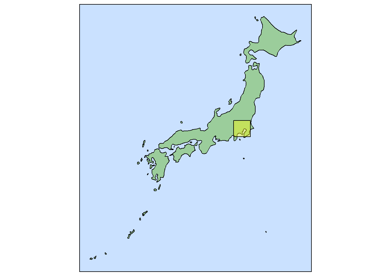
The following example uses a Japan map as the reference. The locations of botanical gardens in the Tokyo region are used to create a basemap (called garden_map). The area shown on the garden_map is used to create an overlay on the Japan map (called JP_overlay). These two maps work together.

Note that if there are any data changes, such as adding a few more gardens to the set of data, both of the maps will be changed automatically. This is a big advantage over the manual specification of the bounding box shown as an overlay on a reference map.

## Some interesting gardens in the Tokyo region.
gardens <- readr::read_csv(file =
"Garden,                      text,        lat,     lon
 Koishikawa Botanical Garden,   Koishikawa,  35.7022,   139.7644
 Jindai Botanical Garden,       Jindai,      35.6726,   139.5643
 Kiyosumi Teien Garden,       Kiyosumi,    35.6797, 139.7987
 Tonogayato Gardens,            Tonogayato,  35.7075,   139.4682
 Kyu-Furukawa Gardens,        Kyu-Furukawa, 35.7347,    139.7393")

## Show the data.
gt(gardens) |>
  fmt_number(
    columns  = c(lat,lon), 
    decimals = 5) |> 
  tab_caption(caption = "Tokyo Botanical Gardens") |>
  tab_source_note(source_note="Source: Gemini AI query")

Tokyo Botanical Gardens

Garden	text	lat	lon
Koishikawa Botanical Garden	Koishikawa	35.70220	139.76440
Jindai Botanical Garden	Jindai	35.67260	139.56430
Kiyosumi Teien Garden	Kiyosumi	35.67970	139.79870
Tonogayato Gardens	Tonogayato	35.70750	139.46820
Kyu-Furukawa Gardens	Kyu-Furukawa	35.73470	139.73930
Source: Gemini AI query

## Extract Japan from the database.
JP <- map_data("world", region = "Japan")

## Make a reference map of Japan.
JP_map <- region_plot(region = JP, coord=1.2)

## Adjust the basemap (garden_map) coverage for labels.
column$margin <- 0.95

## Create a cut-out map using the garden data.
cutout <- site_google_basemap(datatable = gardens)

## Create the garden map with data points and labels.
garden_map <- ggmap(cutout) +
  site_labels(datatable = gardens) +
  site_points(datatable = gardens) +
  simple_black_box 

## Plot the garden map
garden_map

## Extract the bounding box from the cutout.
over_poly <- gmap_bb(gmap=cutout)

## Create the country map with the polygon overlay.
JP_overlay <- JP_map +
  geom_polygon(data=over_poly,
               aes(x = lon, 
                   y = lat,
                   group=1), 
               fill  = "yellow", 
               color = "black",
               alpha = 0.4) +
  island_map_theme

## Plot the map.
JP_overlay