Let’s jump in and make a map before we discuss the map-making process.
What is emphasized here is demonstrating how we can get an adequate map with as little difficulty as possible.
General Setup & Initialization
We need to load some R packages and initialize these as libraries. Table 1 lists the basic R packages that we’ll use. There are other packages that you’ll need later. For now, we’ll focus on this basic set.
The next step is to activate the Google Maps API key. This key provides access to Google Maps.
The key registration needs to be done only once for an RStudio session. This is why the process is kept in a separate R chunk so we don’t keep re-registering as we refine the maps.
Show the code chunk
## Basic Packageslibrary(readr) ## Read in datalibrary(ggmap) ## Show maps, handle Google keylibrary(dplyr) ## Data wranglinglibrary(gt) ## Tableslibrary(ggplot2) ## Build mapslibrary(sitemaps) ## Functions to help build site maps## Mermaid Package (using DiagrammeR)library(DiagrammeR)## Build a table of the key R packagespackages <-read_csv(col_names =TRUE, file ="package, function readr, Read in CSV data in a convenient format ggmap, Help build basemaps, display maps and handle the Google Map key dplyr, Data wrangling gt, Table maker ggplot2, The key to building layered maps tibble, Helps with data frames sitemaps, A set of functions that use table data to build data-based maps")## Print out the package informationgt(packages) %>%tab_style(style =cell_text(v_align ="top"),locations =cells_body())
Table 1: Basic R packages for sitemaps.
package
function
readr
Read in CSV data in a convenient format
ggmap
Help build basemaps, display maps and handle the Google Map key
dplyr
Data wrangling
gt
Table maker
ggplot2
The key to building layered maps
tibble
Helps with data frames
sitemaps
A set of functions that use table data to build data-based maps
Show the code chunk
## Initialize Google Map key; the key is stored in a Project directory. My_Key <-read_file("P://Hot/Workflow/Workflow/keys/Google_Maps_API_Key.txt")## Test if Google Key is registeredif (!has_google_key()){## Register the Google Maps API Key.register_google(key = My_Key, account_type ="standard") } ## end Google Key test
There is also some setup code that needs to be loaded. This is another pretty much standard code block that you’ll need.
What you’re doing is initializing a lot of standard parameters that control details of the appearance of the maps.
Show the code chunk
## Use two functions from sitemaps to initialize parameterscolumn <-site_styles()hide <-site_google_hides()## Establish a theme that improves the appearance of a map.## This theme removes the axis labels and ## puts a border around the map. No legend.simple_black_box <-theme_void() +theme(panel.border =element_rect(color ="black", fill=NA, size=2),legend.position ="none")
It is always a good idea to test a package before going into it too deeply. That’s what we’ll do here.
Our test is a simple map problem: locate the benchmark monuments near downtown Honolulu. A benchmark is a carefully surveyed point. These are reference marks for other surveys. The monument consists of a metal plate on which you’ll find information about the location. The benchmark system also has on-line information that provides more details.
For us, this survey system is handy as the locations of the benchmarks can be copied from an on-line listing.
Step 1: Prepare the Data Table
The data for our map come as a set of comma-separated values (CSV). This is a handy format that is widely used. The read_csv function from the readr package makes the data into a data frame.
Our data frame has quite a bit of information. That’s expected as tables are often used to store relevant data for each of the observations. A table with a lot of data is good as this represents knowledge about each of the places that will be mapped.
Note that in the data in the code chunk looks a bit messy. That’s because the data were cut and pasted from the on-line file … there was no typing. Printing out the data (Table 2) show the values more neatly.
As noted before, there is a lot of data in the table. This is useful for the person using the benchmark data. Here, we’re focused on just three columns: Ref, Lat, and Lon. That’s enough to show how to make a basic map.
Having the proper column names is essential. In order to use the data in our data table, we need to make the following changes:
Ref needs to be made into text so that it will appear in a data-point label.
Lat and Lon need to be shifted to lower case.
We’ll make these two changes with the dplyr::rename function.
Show the code chunk
## Read in the databenchmarks <-read_csv(col_names =TRUE, file ="Ref,Designation,Lat,Lon,Agency,Substrate,Alt-Name,MLLW,MHW1, 161 2340 BM 8, 21.30519,-157.86397,USGS, Concrete bulkhead,B.M. ELV. 8.06 FEET,2.573,2.1342, 161 2340 TIDAL 2, 21.30553,-157.85983,HGSD, Stone pilaster base,161 2340 TIDAL 2,5.185,4.7463, 161 2340 TIDAL 11,21.30575,-157.86389,USCGS,Concrete foundation,NO 11 1925,1.836,1.3974, 161 2340 TIDAL 12,21.30631,-157.86036,USCGS,Concrete floor,NO 12 1925,3.992,3.5525, 161 2340 TIDAL 13,21.30569,-157.85792,USCGS,Concrete floor,NO 13 1925,6.064,5.6256, 161 2340 TIDAL 14,21.30681,-157.85903,USCGS,Concrete balustrade,NO 14 1925,5.495,5.0557, NO 20 1960, 21.30333,-157.86467,USCGS,Concrete pier,NO 20 1960,1.892,1.4538, NO 21 1964, 21.30383,-157.86367,USCGS,Concrete bulkhead,NO 21 1964,2.293,1.8539, GSL 2340 1987, 21.30392,-157.86289,NGS, Concrete pier,GSL 2340 1987,1.872,1.43310,2340 A 1983, 21.30458,-157.86342,NOS, Stainless steel rod,2340 A 1983,1.962,1.52211,2340 B 1983, 21.30670,-157.86700,NOS, Concrete foundation,2340 B 1983,2.706,2.26712,2340 C 1983, 21.30542,-157.86061,NOS, Stainless steel rod,2340 C 1983,2.979,2.53913,161 2340 GPS Bolt,21.30333,-157.86453,HSLC, Metal mast,161 2340 GPS Bolt,5.297,4.858") ## Show the data tablebenchmarks %>%gt() %>%fmt_number(columns =c(Lat,Lon), decimals =5) %>%tab_style(style =cell_text(v_align ="top"),locations =cells_body()) %>%tab_source_note(source_note ="Data: https://tidesandcurrents.noaa.gov/benchmarks.html?id=1612340")
Table 2: Raw data for downtown Honolulu benchmarks.
## Substitute the column names & shift all to lowercasebenchmarks2 <- benchmarks %>% dplyr::rename(text = Ref) %>% dplyr::rename_with(tolower)
Step 2: Build the Basemap
We need a basemap that covers the area with the data locations. The site_google_basemap uses the coordinate information (lat, lon) in the data table to center the basemap and to scale it to the correct size.
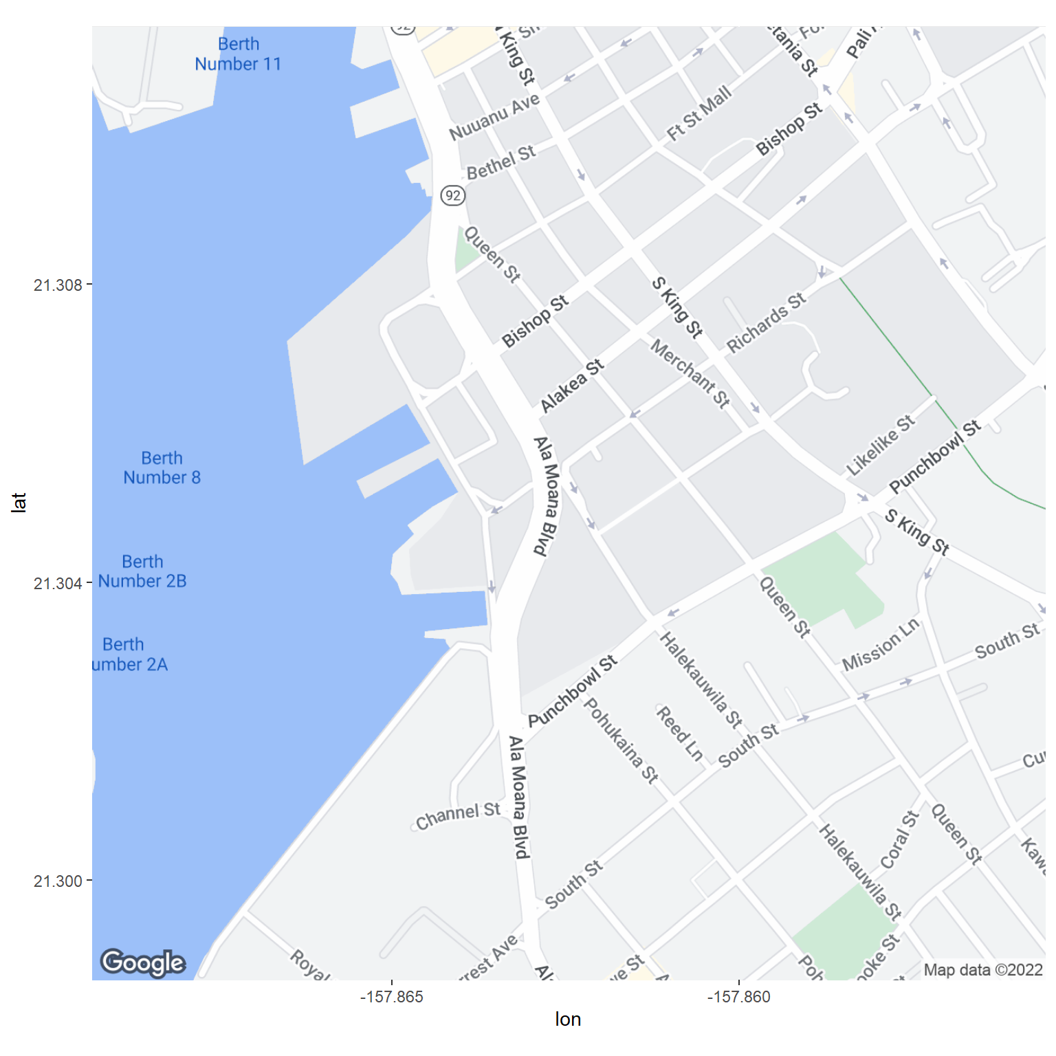
Getting the basemap is the next step. Usually, you don’t need to look at this map. But we’ll show it here as Figure 1.
Show the code chunk
## Adjust a style column valuecolumn$margin <-0.1## Generate a basemapbasemap <-site_google_basemap(datatable = benchmarks2)ggmap(basemap)
Figure 1: Downtown Honolulu basemap.
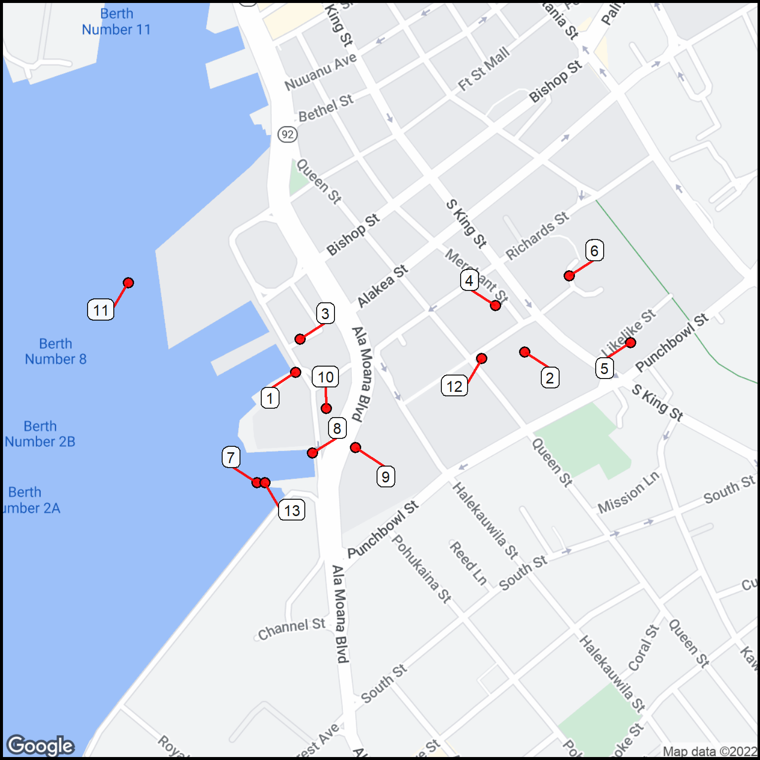
Step 3: Overlay Points and Labels
The final step is to place point markers at each of the benchmark locations. We also want to label each point with a label so we can tie the location back to the data table.
## Show the map (with points & labels)ggmap(basemap) +site_points(datatable = benchmarks2) +site_labels(datatable = benchmarks2) + simple_black_box
Figure 2: Benchmarks in Downtown Honolulu.
At this point, we have confidence that the system is producing maps using our data.
In terms of workflow, note that there was some data wrangling needed to get the column names correct. A style parameter also needed to be modified. But after that, getting a basemap and an overlay with points and labels was quite straightforward. The more complex part had to do with getting the data table configured. Producing the map from there was almost cut-and-paste.
But there was that one parameter change. That was important as it was a style modification. The sitemaps package comes with many default styles. Things like the color of the data points and the size of the labels. You’ll see in the other examples how to use these style modifiers to add information to the map and to make it better suit your needs.
In Summary
We’ve gone through a three-step process in creating a map from a data table (Figure 3). These are the steps that are used over and over in the examples.
The important point is that everything starts with a datatable that has specific column names (e.g., text for the label names, lon and lat for the geographic coordinates).
We’ll soon be adding enhancements to the maps, such as changing the color of the marker points. This will be a simple extension of the process we used here.
Show the code chunk
mermaid(diagram="
  graph LR

  A[datatable]
  B[basemap]
  C[map render]
  D(data: text, lon, lat)
  J(style columns)
  E(site_google_basemap)
  F(ggmap)
  G(site_points)
  H(site_labels)
  style A fill:#2e2,stroke:#000,stroke-width:4px
  style B fill:#2e2,stroke:#000,stroke-width:4px
  style C fill:#2e2,stroke:#000,stroke-width:4px
  subgraph
  A ==> E
  B ==> F
  D -.-> A
  E -.-> B
  J -.-> A
  F -.-> C
  G -.-> C
  H -.-> C
  A ==> G
  A ==> H
  end")
Figure 3: The three-step process of map creation.
Looking Ahead
Consider that the table gives you the details. The map shows not only the geographic locations, but you can also see relationships inherent in the data. Maps and tables fit together well, each bringing a complementary strength to the relationship.
Maps can be simple or complex. Manipulation of the symbolism features involves adding columns to the data table. Most of the effort is in getting the data in order. But you’ll also want to examine how map symbolism (e.g., point color, point outline, point size) can add interesting additional information to the map.
A Bit More About R Packages
There are quite a few R packages that are useful, sometimes essential, for the map-making process beyond those that are essential (Table 1). These supplemental packages are shown in Table 3.
These following packages will be highlighted in the descriptions of the sitemaps functions that require their use.
Show the code chunk
morelibs <-read_csv(col_names =TRUE, file ="Package, Use geosphere, Distance and direction calculations sp, Spatial point data structure conversion and processing parzer, Convert HMS to digital coordinates jsonlite, Process files using the JSON format httr, Allow API calls")gt(morelibs)%>%tab_style(style =cell_text(v_align ="top"),locations =cells_body())
Table 3: Additional R packages used with sitemaps.
Package
Use
geosphere
Distance and direction calculations
sp
Spatial point data structure conversion and processing