Sitemaps: The Website - Getting Locations

Placing data points, labels and names on a map requires the specification of location information. Generally, we thing of using geographic coordinates, like latitude and longitude. These values work, but they are often hard to get and tedious to enter. Ahhh … so many digits to type.

Important

Avoid retyping coordinate data to the maximum extent possible. Download the values or do a copy-paste.

First, lets set up the libraries and setup code.

Show the code chunk

## Libraries
library(readr)        ## Read in data
library(ggmap)        ## Show maps, handle Google key
library(ggplot2)      ## Build maps
library(dplyr)        ## General data wrangling
library(gt)           ## Tables
library(sitemaps)     ## Functions to help build site maps
library(parzer)       ## Convert HMS to digital coordinates
library(lubridate)    ## Handle times and dates in wonderful ways
library(exifr)        ## Get photo EXIF data
library(stats)        ## Help to initialize files
library(tibble)       ## Add columns function

## Initialize Google Map key; the key is stored in a Project directory.
  My_Key <- read_file("P://Hot/Workflow/Workflow/keys/Google_Maps_API_Key.txt")

## Test if Google Key is registered
if (!has_google_key()){

  ## Register the Google Maps API Key.
  register_google(key = My_Key, account_type = "standard")
  } ## end Google Key test

The standard setup code chunk follows.

Show the code chunk

## Use two functions from sitemaps to initialize parameters
column <- site_styles()
hide  <- site_google_hides()

## Establish a theme that improves the appearance of a map.
## This theme removes the axis labels and 
## puts a border around the map. No legend.
simple_black_box <- theme_void() +
              theme(panel.border = element_rect(color = "black", 
                                   fill=NA, 
                                   size=2),
                    legend.position = "none")

Latitude & Longitude Formats

Most newer publications use a digital (i.e., ddd.ddddd) representation of each geographic coordinate. Many places you find data will use this format. If you are recording your own data values, for example with a cell-phone, you should use this digital format.

The functions used here almost always use the decimal digits format.

But sometimes, you get data in the hours, minutes and seconds format (hh mm ss). To make matter worse, this format comes with a number of variations.

Never fear! There are ways to read a whole variety of formats and convert them to the decimal format. Take a look at the format challenges in Table 1.

Show the code chunk

## Note that there are subtle differences between the 
## single and double quote marks.
landmarks <- read_csv(col_names = TRUE, file = 
        "alat,            alon,           name
        48°51′29.6″N,     2°17′40.2″E,    Eiffel Tower
        48°52′25.67″N,    2°17′42.04″E,   Arc de Triomphe
        48.8530°N,        2.3498°E,       Notre-Dame de Paris
        48.88686,         2.34303,        Sacré-Cœur
        48° 51′ 39.07″ N, 2° 20′ 8.92″ E, Louvre Palace
        48:51:36 N,       2:19:35 E,      Musée d'Orsay
        48 51 19 N,       2 20 42 E,      Sainte-Chapelle")

## Convert the coordinates.
landmarks = landmarks %>%
  mutate(lon = parzer::parse_lon(alon),
         lat = parzer::parse_lat(alat))

## Print a table with the data.
gt(landmarks) %>% 
  fmt_number(columns = c(lat,lon), decimals = 5)

Table 1: Different formats converted to the digital format.
alat	alon	name	lon	lat
48°51′29.6″N	2°17′40.2″E	Eiffel Tower	2.29450	48.85822
48°52′25.67″N	2°17′42.04″E	Arc de Triomphe	2.29501	48.87380
48.8530°N	2.3498°E	Notre-Dame de Paris	2.34980	48.85300
48.88686	2.34303	Sacré-Cœur	2.34303	48.88686
48° 51′ 39.07″ N	2° 20′ 8.92″ E	Louvre Palace	2.33581	48.86085
48:51:36 N	2:19:35 E	Musée d'Orsay	2.32639	48.86000
48 51 19 N	2 20 42 E	Sainte-Chapelle	2.34500	48.85528

You should see from this example that most of the coordinate formats can be converted with the use of the parzer functions.

Making sure your data are in a digital format is one of the first steps in data wrangling.

Getting Geographic Coordinates

There are quite a few strategies. Which one works for you depends on your problem. The following are some suggestions.

You need to use the decimal values for all the coordinates. In some situations, you’ll likely need to change the options for your device or software to get the decimal format.

Five decimal digits is enough precision. This corresponds to values close to 1 meter resolution.

Copy From Existing Digital Sources

You can often find digital location using Internet resources. Wikipedia, for example, frequently lists the geographic coordinates of places for which there is an article. This is often in small type in the upper right hand corner.

Remember that you should try to copy and paste instead of retyping the values.

Locations from Google Maps

Running Google Maps helps you get the needed information for all these location requirements. If you use this strategy, you’ll quickly find the data you need and you will never need to write down and type all the location numbers.

Locate the area on Google Maps in a browser.
Get the coordinates of a point (either a central location or corner) by right-clicking a location point.
The point coordinates appear at the top of a pop-up menu.
Left-click on the coordinates values and they will be put in the copy buffer.
Paste the coordinates into the R code chunk with CTRL-V.

Note that the order of the coordinates given by Google is Latitude, Longitude. The mapping done here requires it the other way around (Lon,Lat). See the warning below.

Warning

When you provide data for Google Maps, you need to give the coordinates in the proper order. Longitude always comes first in the specifications.

An easy way to remember this is that the corners are given as (x,y) pairs (aka “Cartesian coordinates”). The longitude is x and latitude is y.

When you retrieve values from a Google map, the coordinates are given in the (latitude, longitude) order and, therefore, the values need to be transposed.

Geocode Place Names & Addresses

If you have buildings (e.g., residences, institutions, businesses) as your locations, you can do a reverse geocode to get the coordinates. This works surprisingly well for many locations around the world.

If you’re interested in finding a place, you might check the website geonames.org. It currently has more than eleven million place names in its worldwide database.

The geocode function requires the use of a Google Maps key. It is the same key you use for making Google Maps.

Table 2 shows some place names that have been converted using the geocode function.

Show the code chunk

## Reset the parameters
column <- site_styles()

## Read the data
inst <- read_csv(col_names = TRUE, file = 
    "place,                   city,      country
    玉川大学教育博物館,       Tokyo,     Japan
    Chelsea Physic Garden,    London,    England
    Royal Botanical Garden,   Kolkata,   India
    University of Cape Town,  Cape Town, Union of South Africa
    北京植物园,               Beijing,   PRC")

## Combine the location information.
location <- paste0(inst$place,", ",inst$city, ", ", inst$country) 

## Get the coordinates from the location.
coord <- geocode(location, output = "latlon")

## Add the coordinates to the original location data.
inst <- cbind(inst,coord)

gt(inst) %>% 
  fmt_number(columns = c(lat,lon), decimals = 5)

Table 2: Locations with place names.
place	city	country	lon	lat
玉川大学教育博物館	Tokyo	Japan	139.47243	35.56937
Chelsea Physic Garden	London	England	−0.16290	51.48488
Royal Botanical Garden	Kolkata	India	88.29112	22.55869
University of Cape Town	Cape Town	Union of South Africa	18.46120	−33.95765
北京植物园	Beijing	PRC	116.21083	39.99132

On Site Recording: GPS Software & Photo Metadata

You can collect location coordinates when you collect field data. A while ago, you needed a dedicated GPS receiver to get the coordinates. Now, there are many apps that use a phone’s GPS capabilities to receive and record location coordinates.

A generally overlooked alternative is to simply take a photo at the point you want to record the location. Most cell phones, for example, will put the location into the metadata. Make sure that the phone options allow this before you depend on this form of data recording.

Once you’ve collected some location images, you probably want to edit the photos (using a metadata editor) include some message in the image (e.g., “site 22”).

You can extract the photo location and description values for each photo using the site_photos function. This function assumes that all the images are in a folder.

The following code chunk is an example that reads all the photos in a folder and retrieves the location coordinates. The result is Table 3.

Show the code chunk

## Reset the parameters
column <- site_styles()

## Retrieve the EXIF data from the JPG photos in the folder
photo_table <- site_photos("photos/HotSpot")

## Put out a table to confirm the EXIF data
gt(photo_table) %>% 
  fmt_number(columns = c(lat,lon), decimals = 5)

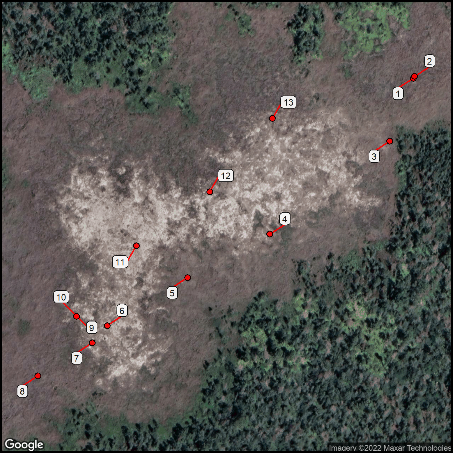
Table 3: Information from the JPG images at the Puhimau Hot Spot.
number	file	description	lat	lon	dir	dist	date	time
1	IMG_20170701_104924.jpg	Site 01	19.38983	−155.24857	0	2	2017-07-01	10:49
2	IMG_20170701_104956.jpg	Site 02	19.38985	−155.24856	296	1	2017-07-01	10:49
3	IMG_20170702_095342.jpg	Site 03	19.38938	−155.24875	197	1	2017-07-02	9:53
4	IMG_20170702_095843.jpg	Site 04	19.38872	−155.24966	211	1	2017-07-02	9:58
5	IMG_20170702_100351.jpg	Site 05	19.38841	−155.25028	199	1	2017-07-02	10:03
6	IMG_20170702_100910.jpg	Site 06	19.38806	−155.25089	113	2	2017-07-02	10:09
7	IMG_20170702_101659.jpg	Site 07	19.38794	−155.25101	247	1	2017-07-02	10:17
8	IMG_20170702_102434.jpg	Site 08	19.38771	−155.25142	245	1	2017-07-02	10:24
9	IMG_20170702_103046.jpg	Site 09a	19.38813	−155.25113	46	1	2017-07-02	10:30
10	IMG_20170702_103053.jpg	Site 09b	19.38813	−155.25113	135	2	2017-07-02	10:30
11	IMG_20170702_103613.jpg	Site 10	19.38864	−155.25067	284	1	2017-07-02	10:36
12	IMG_20170702_104040.jpg	Site 11	19.38902	−155.25012	281	1	2017-07-02	10:40
13	IMG_20170702_104723.jpg	Site 12	19.38955	−155.24964	286	1	2017-07-02	10:47

We can now show (Figure 1) where the photos were taken with a map based on a satellite image.

Show the code chunk

## Make a text column from the photo number
photo_table$text <- as.character(photo_table$number)

## Use a satellite image for the basemap
column$gmaptype <- "satellite"

## Build the basemap
basemap <- site_google_basemap(datatable = photo_table)

## Create the map
image1 <- ggmap(basemap) +
  site_labels(datatable = photo_table) +
  site_points(datatable = photo_table) +
  simple_black_box

image1