A “fan” is a graphic symbol that shows a location, direction and field width. Combined with the other graphic symbols, the fan places photos in a rich context on base maps.
The basic information for a fan symbol is added to a basic data table or it can be in its own data table. This distinction is important as it is often possible to generate a data table from a set of photographs. The site_photos function builds a table with values you can use to create the fields necessary for the site_fans function. You’ll see how this works in a few examples.
Cellphones collect considerable data about photos being taken. These data values are stored in each photo’s EXIF data which is part of a JPG (or JPEG) image. This shows an advantage of using cellphone photos to document sites. Many “regular” cameras do not store all of the information needed to create fan symbols.
It is possible, although perhaps tedious, to add data if a set of photos doesn’t have location, direction or view width information. In that case, the values used may be general approximation. These are often adequate for the sorts of maps produced with the sitemaps functions.
Getting Started
We’ll get started by doing our usual initialization.
Show the code chunk
library(geosphere)library(sitemaps)library(ggmap)library(ggplot2)library(readr)library(gt)library(dplyr)library(sp) ## To make the SpatialPointslibrary(maptools) ## Used? Going to be retired at end of 2023library(tibble)library(stringr)library(exifr) ## Get photo EXIF datalibrary(lubridate) ## Handle dateslibrary(stats)library(REAT) ## Used to do the regression for the field of viewlibrary(exifr) ## Photo EXIF data retrieval## Initialize Google Map key; the key is stored in a Project directory. My_Key <-read_file("P://Hot/Workflow/Workflow/keys/Google_Maps_API_Key.txt")## Test if Google Key is registered.if (!has_google_key()){## Register the Google Maps API Key.register_google(key = My_Key, account_type ="standard") } ## end Google Key test
A few more things are need before we begin.
Show the code chunk
## Use two functions from sitemaps to initialize parameterscolumn <-site_styles()hide <-site_google_hides()## Establish a theme that improves the appearance of a map.## This theme removes the axis labels and ## puts a border around the map. No legend.simple_black_box <-theme_void() +theme(panel.border =element_rect(color ="black", fill=NA, size=2),legend.position ="none")
Example: Map photos using default values
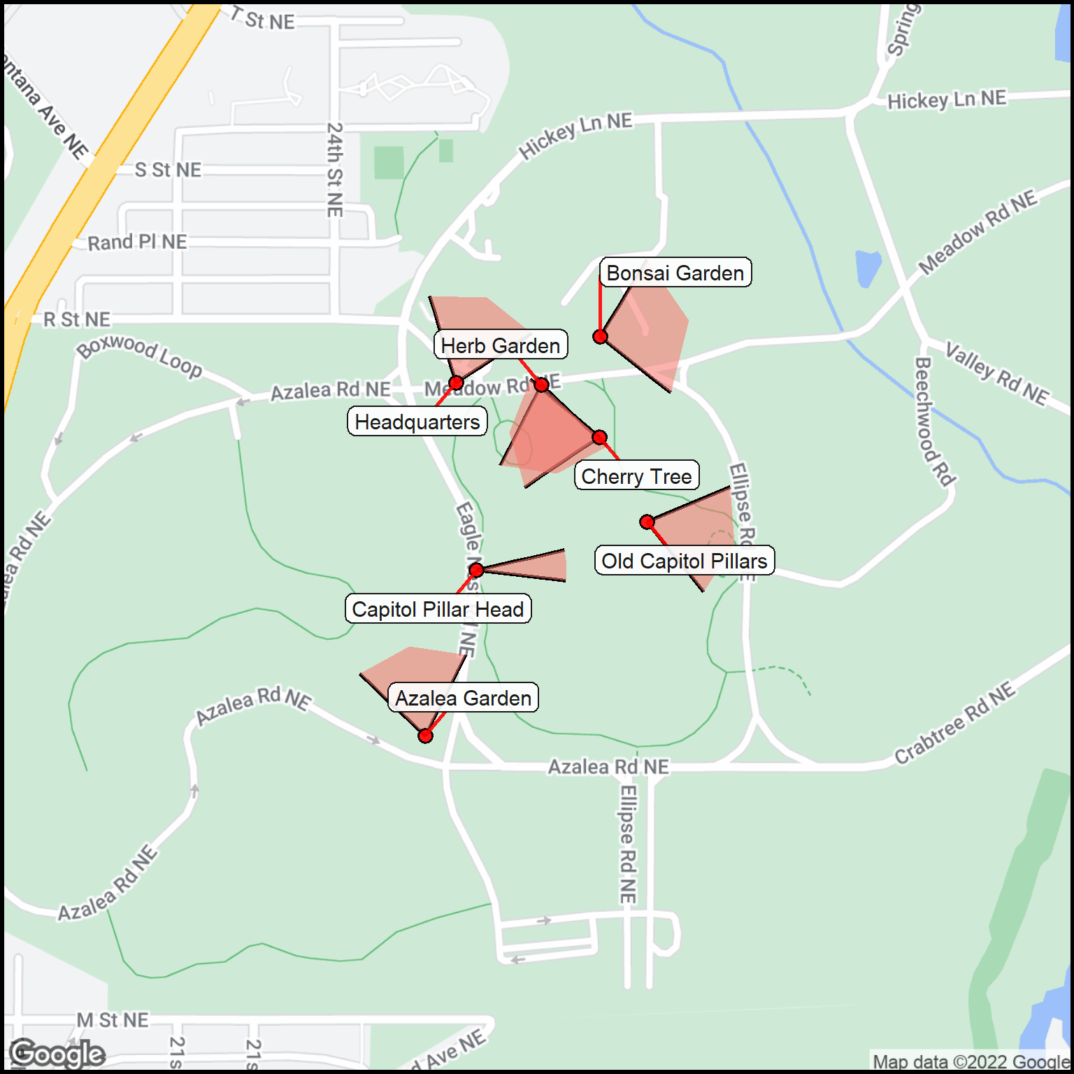
This example shows the locations and direction information for a few photos taken with a cellphone at the National Arboretum (Washington, DC).
All of the data (Table 1) for the map come from an EXIF extraction using the site_photo function. A few columns needed renaming so that they will plot using the site_fans and site_labels functions.
The purpose of this example is to show the relative ease of providing a map with photo information with very little code.
Warning
The dir and fov data in the photo EXIF file may not be accurate, especially if the camera compass is not calibrated. It is possible to manually update the EXIF data using exiftool with the exiftool GUI software. Consult exiftool.org for the software and editing information.
Show the code chunk
## Reset the defaultscolumn <-site_styles()## Photo folderfolder <-"photos/NatArboretum"## Read the EXIF dataexif_data <-site_photos(folder)## Print the data for confirmationgt(exif_data) %>%fmt_number(columns =c(lat,lon), decimals =5) %>%fmt_number(columns = fov, decimals =0)
Table 1: Image information for photos from the National Arboretum.
number
file
description
lat
lon
dir
fov
dist
date
time
1
PXL_20220404_154844253.jpg
Headquarters
38.91195
−76.97059
20
74
3
2022-04-04
11:48
2
PXL_20220404_163353453.jpg
Bonsai Garden
38.91241
−76.96875
80
97
3
2022-04-04
12:33
3
PXL_20220404_165324797.jpg
Herb Garden
38.91193
−76.96950
170
74
3
2022-04-04
12:53
4
PXL_20220404_165931864.jpg
Cherry Tree
38.91141
−76.96876
273
74
3
2022-04-04
12:59
5
PXL_20220404_170448577.jpg
Old Capitol Pillars
38.91056
−76.96815
104
74
3
2022-04-04
13:04
6
PXL_20220404_175915228.jpg
Azalea Garden
38.90844
−76.97099
350
74
3
2022-04-04
13:59
7
PXL_20220404_180736978.jpg
Capitol Pillar Head
38.91008
−76.97033
87
20
3
2022-04-04
14:07
The photo file has been processed and returned relevant information. However, the site_photos function purposely returns column names that are not correct for processing with the site_fans function. This is done because it isn’t always obvious which columns will be used and, quite possibly, how they should be modified before they are used.
The next code chunk shows a simple renaming of the key columns and the production of a map (Figure 1) with the fan symbols.
Show the code chunk
## Save a new dataset with column names updated so they are standard.exif_data2 <- exif_data %>% dplyr::rename(text = description, fan_direction = dir, fan_field_width = fov)## Adjust the basemap margincolumn$margin <-0.8## Basemapbasemap <-site_google_basemap(datatable = exif_data2)## Put on data points, labels and armsfan_test <-ggmap(basemap) +site_fans(datatable = exif_data2) +site_points(datatable = exif_data2) +site_labels(datatable = exif_data2) + simple_black_boxfan_test
Figure 1: Fan symbols for photos taken at the National Arboretum.
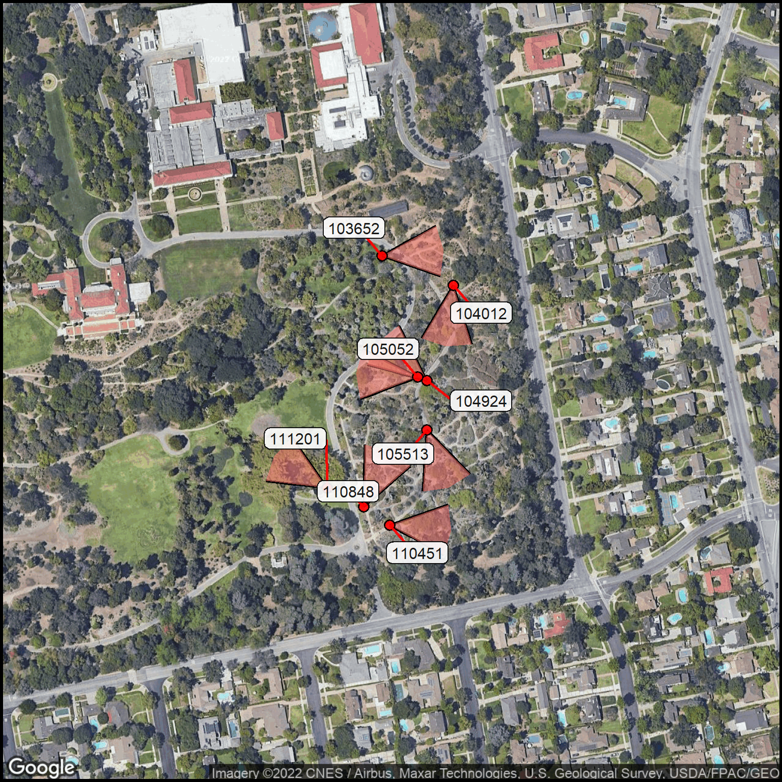
Example: Adding direction data to photo locations
Some cell phones (and maybe cameras) provide both the direction (bearing) and view width (FOV) for each photo with this information saved in the EXIF data.
This example, photo information only had the lat/lon data. This was copied into the data table. Reference to a Google Maps image provided an estimation of the direction each photo was taken. Table 2 provides another test of the sites_fan function.
Show the code chunk
## Reset the parameterscolumn <-site_styles()## The data file with the photo direction informationdirection_data <-read_csv(col_names =TRUE, file ="text, lat, lon, fan_direction103652, 34.126966, -118.110479, 85104012, 34.126753, -118.109852, 187104924, 34.126059, -118.110084, 309105052, 34.126086, -118.110165, 273105513, 34.125702, -118.110084, 160110451, 34.125009, -118.110411, 95110848, 34.125142, -118.110639, 25111201, 34.125277, -118.110960, 301")## Put out a table to confirm the EXIF datagt(direction_data) %>%fmt_number(columns =c(lat,lon), decimals =5)
Table 2: Image information for photos from the Huntington Botanical Garden.
text
lat
lon
fan_direction
103652
34.12697
−118.11048
85
104012
34.12675
−118.10985
187
104924
34.12606
−118.11008
309
105052
34.12609
−118.11016
273
105513
34.12570
−118.11008
160
110451
34.12501
−118.11041
95
110848
34.12514
−118.11064
25
111201
34.12528
−118.11096
301
The data table already has the correct names for the site_fans and site_labels functions. Now it is time to do a plot on a satellite image (Figure 2).
The code chunk has a commented-out statement that shows how to get a PNG file with the map.
Show the code chunk
# ## Rename some columns to the standard names# photo_exif2 <- photo_exif %>% # dplyr::rename(text=number, fan_direction=dir, fan_field_width=fov)## Adjust some of the fan stylescolumn$fan_alpha <-0.4column$fan_arm_length <-50column$margin <-0.9## Assign a field width based on the camera information (lens length, etc)## This is the same for all the photoscolumn$fan_field_width <-48## Basemapcolumn$gmaptype <-"satellite"basemap <-site_google_basemap(datatable = direction_data)## Put on data points, labels and armsplot_hunt <-ggmap(basemap) +site_fans(datatable = direction_data) +site_points(datatable = direction_data) +site_labels(datatable = direction_data) + simple_black_boxplot_hunt## ggsave(filename="Huntington_photolocs.png",plot=plot_hunt, width=8, height=8)
Figure 2: Photos in the desert area at the Huntington Botanical Garden
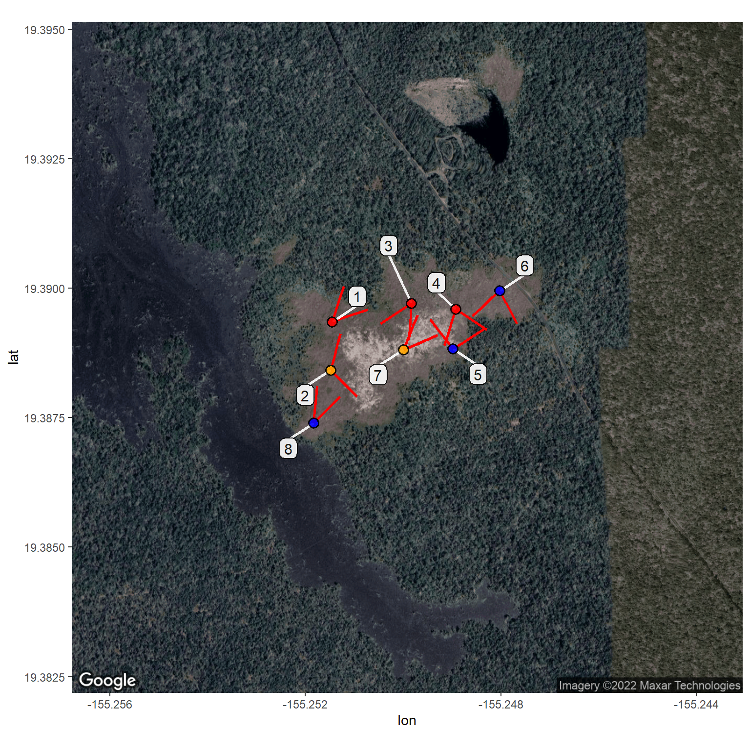
Example: Fan symbols and point colors
This example is a reminder that the other sitemap functions can be used with the fan symbols.
We’ll use site_fans function with the Puhimau map to show the locations, directions and field of view of each of the photos taken at this research site along with the a color code to indicate the temperature category. The analysis starts with just the location and temperature data (Table 3).
Show the code chunk
## Read in the field data.puhimau <-read_csv(col_names =TRUE, file ="Site, Lon, Lat, Temperature, color 1, -155.251451, 19.389354, 140, red 2, -155.251483, 19.388421, 125, orange 3, -155.249834, 19.389709, 165, red 4, -155.248924, 19.389591, 180, red 5, -155.248982, 19.388827, 102, blue 6, -155.248024, 19.389952, 97, blue 7, -155.249994, 19.388816, 135, orange 8, -155.251831, 19.387395, 95, blue")## Rename the a few column and shift all the column names to lowercasepuhimau2 <- puhimau %>% dplyr::rename(text = Site, point_color = color) %>% dplyr::rename_with(tolower)## Show the data in a tablegt(puhimau2) %>%fmt_number(columns =c(lat,lon), decimals =5) %>%tab_source_note(source_note ="Data: 2017 field survey") %>%tab_footnote(footnote ="degrees F",locations =cells_column_labels(columns = temperature))
Table 3: Surface soil temperature measurements at Puhimau Hot Spot.
text
lon
lat
temperature1
point_color
1
−155.25145
19.38935
140
red
2
−155.25148
19.38842
125
orange
3
−155.24983
19.38971
165
red
4
−155.24892
19.38959
180
red
5
−155.24898
19.38883
102
blue
6
−155.24802
19.38995
97
blue
7
−155.24999
19.38882
135
orange
8
−155.25183
19.38740
95
blue
Data: 2017 field survey
1 degrees F
The next thing is to add some data specifically for the fans. The two key items are the fan_direction (bearing) of the photo and the fan_field_width (field of view).
A new data table is constructed that has the fan information. The tables are merged with the column that is the same in both tables (“text”). As usual, it is a good idea to check that all is well (Table 4) before moving on.
Show the code chunk
## Read the extra data about the photosphoto_dir <-read_csv(col_names =TRUE, file ="text, fan_direction, fan_field_width 1, 45, 53 2, 75, 120 3, 210, 53 4, 160, 75 5, 10, 95 6, 190, 75 7, 45, 45 8, 25, 40")## Merge the two sets of datapuhimau3 <-merge(puhimau2, photo_dir, by="text") ## Make a table to verify the datagt(puhimau3) %>%fmt_number(columns =c(lat,lon), decimals =5)
Table 4: Full data for the Puhimau photo locations.
text
lon
lat
temperature
point_color
fan_direction
fan_field_width
1
−155.25145
19.38935
140
red
45
53
2
−155.25148
19.38842
125
orange
75
120
3
−155.24983
19.38971
165
red
210
53
4
−155.24892
19.38959
180
red
160
75
5
−155.24898
19.38883
102
blue
10
95
6
−155.24802
19.38995
97
blue
190
75
7
−155.24999
19.38882
135
orange
45
45
8
−155.25183
19.38740
95
blue
25
40
We’re now ready to place the fan symbols on the map (Figure 3). Note that a few of the default values for the fan have been changed.
Show the code chunk
## Modify the arm characteristics & don't fill the fancolumn$fan_arm_length <-80column$fan_arm_color <-"red"column$fan_fill <-FALSE## Modify the label connector color so that it isn't confused with the armscolumn$label_connector_color <-"white"## Obtain a basemapcolumn$gmaptype <-"satellite"basemap <-site_google_basemap(datatable = puhimau3)## Put on data points, labels and fan armspuhi_map <-ggmap(basemap) +site_fans(datatable = puhimau3) +site_labels(datatable = puhimau3) +site_points(datatable = puhimau3)puhi_map
Figure 3: Photo locations and view areas at Puhimau Hotspot.
Calculating the Field of View
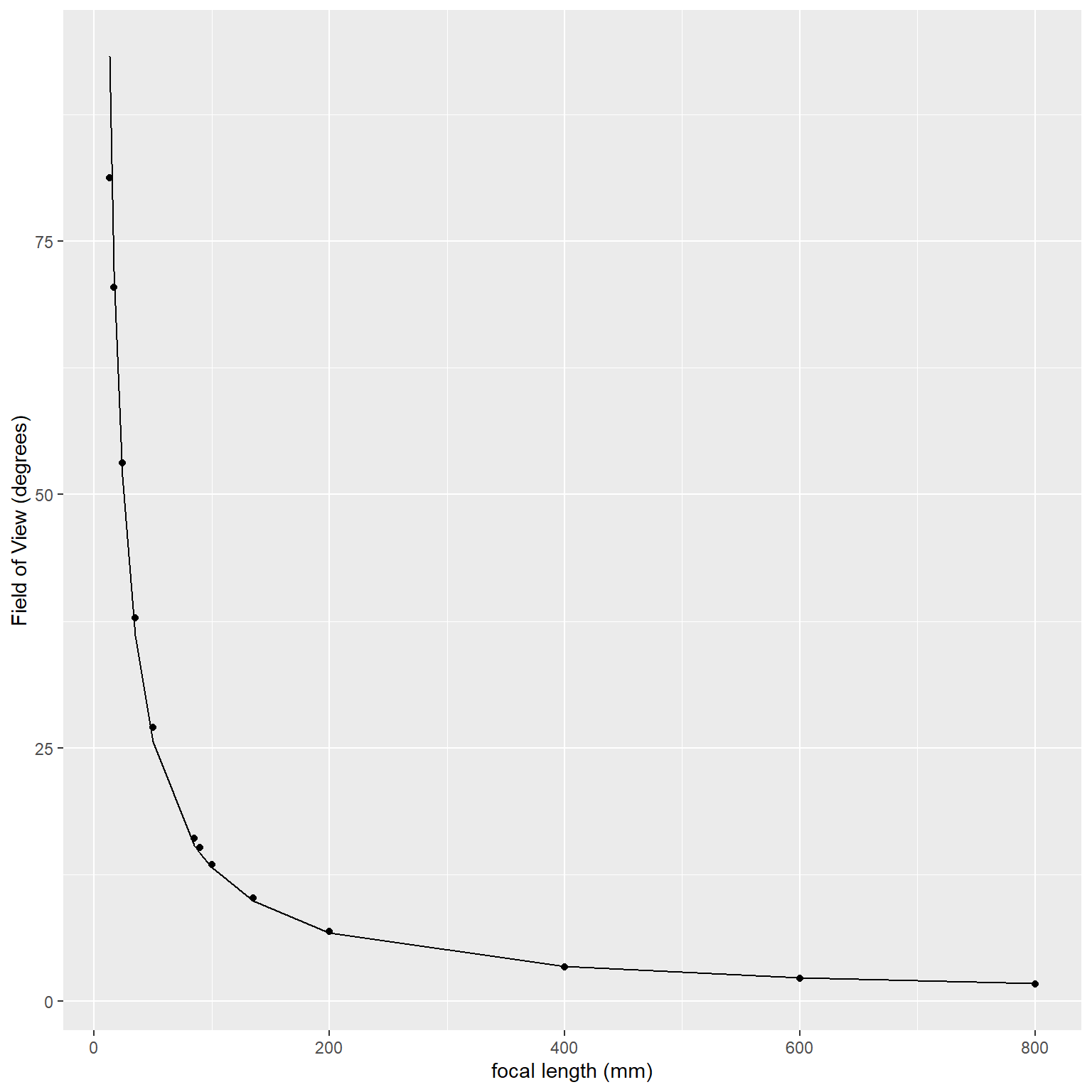
The field of view of a camera, which is used as the fan_field_width, depends on the focal length of the lens and the sensor size. For the discussion here, let’s assume we are working with full-frame (or equivalent) camera sensors.
Data relating the field of view to the lens focal length is given at the www.nikonians.org/reviews/fov-tables website. The data from this website are used here to develop a function that can be used to calculate the field of view from the focal length.
The function is:
field of view <- 1088.15264 * focal_length ^ -0.95814
The function works pretty well except as the shortest focal lengths. Nonetheless, this is probably adequate for the diagrams produced by site_fans.
The code a function that can be used to calculate the horizontal field of view for any lens using the focal length (mm).
Show the code chunk
## Field of View datafov <-read_csv(col_names =TRUE, file ="focal_length, horiz_fov 13, 81.2 17, 70.4 24, 53.1 35, 37.8 50, 27.0 85, 16.1 90, 15.2100, 13.5135, 10.2200, 6.9400, 3.4600, 2.3800, 1.7")## Get the fit to several popular regression modelsparms <-curvefit(fov$focal_length, fov$horiz_fov, plot.curves =FALSE)
Curve fitting

                       a            b Std. Error a Std. Error b   t value a
Linear        38.9727451 -0.065847661   7.85888900 0.0253613157   4.9590655
Power       1088.1526430 -0.958140163   0.02523186 0.0123547203 120.3514143
Exponential   34.5382982 -0.004531752   0.21212657 0.0006845508  16.6979022
Logistic      -0.5874711  0.007211284   0.81927038 0.0026438565  -0.7170662
             t value b   Pr(>|t|) a   Pr(>|t|) b R squared Adj. R squared
Linear       -2.596382 4.294222e-04 2.485382e-02 0.3799743      0.3236083
Power       -77.552558 1.630833e-18 2.039202e-16 0.9981744      0.9980084
Exponential  -6.620038 3.668037e-09 3.760363e-05 0.7993612      0.7811213
Logistic      2.727563 4.882802e-01 1.966383e-02 0.4034577      0.3492266
                F value       Pr(>F)
Linear         6.741199 2.485382e-02
Power       6014.399260 2.039202e-16
Exponential   43.824899 3.760363e-05
Logistic       7.439598 1.966383e-02
Show the code chunk
## The power model works bestparms ## look at power model
$models_comp
                       a            b Std. Error a Std. Error b   t value a
Linear        38.9727451 -0.065847661   7.85888900 0.0253613157   4.9590655
Power       1088.1526430 -0.958140163   0.02523186 0.0123547203 120.3514143
Exponential   34.5382982 -0.004531752   0.21212657 0.0006845508  16.6979022
Logistic      -0.5874711  0.007211284   0.81927038 0.0026438565  -0.7170662
             t value b   Pr(>|t|) a   Pr(>|t|) b R squared Adj. R squared
Linear       -2.596382 4.294222e-04 2.485382e-02 0.3799743      0.3236083
Power       -77.552558 1.630833e-18 2.039202e-16 0.9981744      0.9980084
Exponential  -6.620038 3.668037e-09 3.760363e-05 0.7993612      0.7811213
Logistic      2.727563 4.882802e-01 1.966383e-02 0.4034577      0.3492266
                F value       Pr(>F)
Linear         6.741199 2.485382e-02
Power       6014.399260 2.039202e-16
Exponential   43.824899 3.760363e-05
Logistic       7.439598 1.966383e-02

$models_y
        x    y   ypred_lin ypred_pow  ypred_exp ypred_logi
 [1,]  13 81.2  38.1167256 93.191426 32.5623274 50.4742767
 [2,]  17 70.4  37.8533349 72.068800 31.9773875 49.9205583
 [3,]  24 53.1  37.3924013 51.790964 30.9789129 48.9428657
 [4,]  35 37.8  36.6680770 36.079143 29.4724954 47.3864490
 [5,]  50 27.0  35.6803621 25.635301 27.5356405 45.2317341
 [6,]  85 16.1  33.3756940 15.418285 23.4969318 40.1227029
 [7,]  90 15.2  33.0464557 14.596596 22.9705071 39.3903921
 [8,] 100 13.5  32.3879791 13.195003 21.9527753 37.9286790
 [9,] 135 10.2  30.0833110  9.897636 18.7329169 32.8919003
[10,] 200  6.9  25.8032130  6.791732 13.9533320 24.2567407
[11,] 400  3.4  12.6336809  3.495841  5.6370894  7.4265162
[12,] 600  2.3  -0.5358512  2.370454  2.2773612  1.8872538
[13,] 800  1.7 -13.7053833  1.799379  0.9200447  0.4541876
Show the code chunk
## Power model parametersfov$fit_fov <-1088.15264*fov$focal_length^-0.95814## Check results with a tablegt(fov)
focal_length
horiz_fov
fit_fov
13
81.2
93.191464
17
70.4
72.068833
24
53.1
51.790991
35
37.8
36.079164
50
27.0
25.635317
85
16.1
15.418296
90
15.2
14.596607
100
13.5
13.195013
135
10.2
9.897644
200
6.9
6.791738
400
3.4
3.495844
600
2.3
2.370456
800
1.7
1.799381
Figure 4: Field of view for lenses with different focal lengths.
Show the code chunk
## Look at a plotggplot(fov, aes(x=focal_length, y=horiz_fov)) +geom_point() +geom_line(aes(x=focal_length, y=fit_fov)) +labs(x ="focal length (mm)",y ="Field of View (degrees)")## Here is a function that can be used in some codefield <-function(focal_len){## Field of View approximation fit <-1088.15264*focal_len^-0.95814return(fit)} ## end function field## Test the function with a lens focal lengthfocal_length <-100field <-field(focal_length)test_result <-paste0("A lens with a focal length of ", focal_length, " (mm) has an approximate field of view of ",round(field, digits=1)," (degrees).")cat(test_result)
A lens with a focal length of 100 (mm) has an approximate field of view of 13.2 (degrees).
Figure 5: Field of view for lenses with different focal lengths.