Getting an appropriate basemap is an essential first step in the map making process. The examples shown in this gallery show some of the variety you can get by using fairly simple R code.
Later, you’ll see that the specification of a basemap is made easier by using some functions. Here, we’re only focused on the general appearance of the basemaps. These examples will help you decide what type of basemap will best suit your project.
Setup & Defaults
Setup Information
Each section has its own setup and default information. This allows each section to be run independently. The duplication of code is a small price to be paid for the independence and clarity achieved by this repetition.
All use of Google maps requires the use of an API key. Getting this key is a one-time task. Store the key somewhere same and hidden from the outside.
Registering the Google Key needs to be done once each session.
Show the code chunk
## Librarieslibrary(readr)library(ggmap)library(ggplot2)library(sitemaps)## Initialize Google Map key; the is stored in a Project directory. My_Key <-read_file("P://Hot/Workflow/Workflow/keys/Google_Maps_API_Key.txt")## Test if Google Key is registeredif (!has_google_key()){## Register the Google Maps API Key.register_google(key = My_Key, account_type ="standard") } ## end Google Key test
Some Required and Useful Code
It is essential to include the code to set the parameters (site_styles()) and the Google Map hide codes (site_google_hides()).
This code block also defines a simple theme that removes the geographic coordinates from the map borders, places a black line around the map, and suppresses a default legend.
Show the code chunk
## Read in all the parameterscolumn <-site_styles()hide <-site_google_hides()################################################################### Define a theme that removes the axis labels and ## puts a border around the map. No legend.simple_black_box <-theme_void() +theme(panel.border =element_rect(color ="black", fill=NA, size=2),legend.position ="none")
Google Basemaps
The Google basemaps have annotations on top. There are ways to selectively limit the annotation. This capability is discussed later along with a few other features that make these maps more useful.
Map Type
Appearance
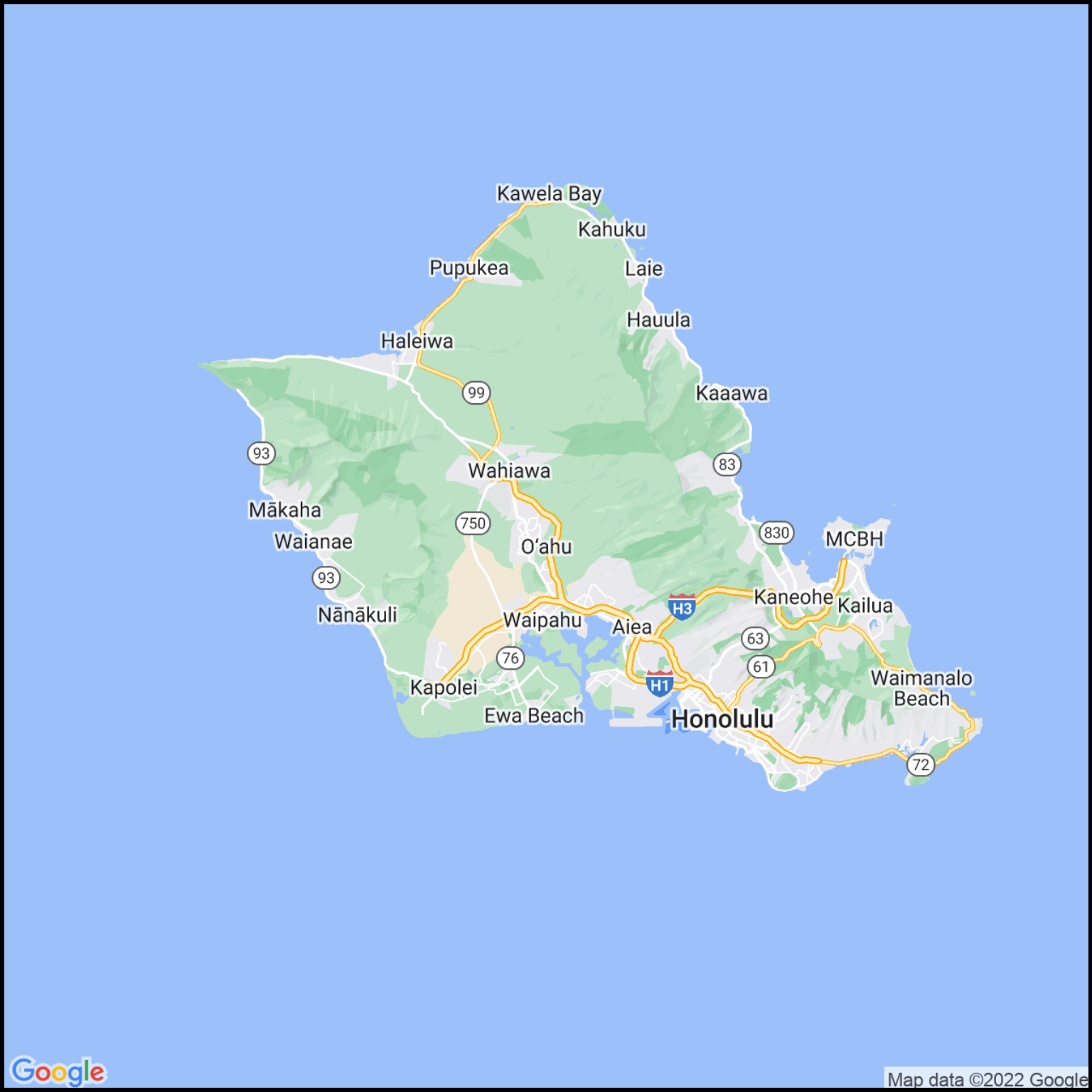
roadmap
Street map
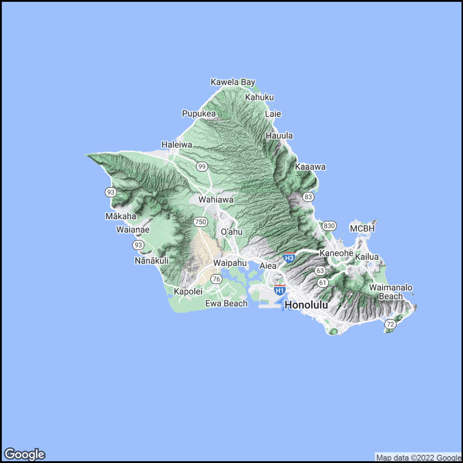
terrain
Shaded relief map
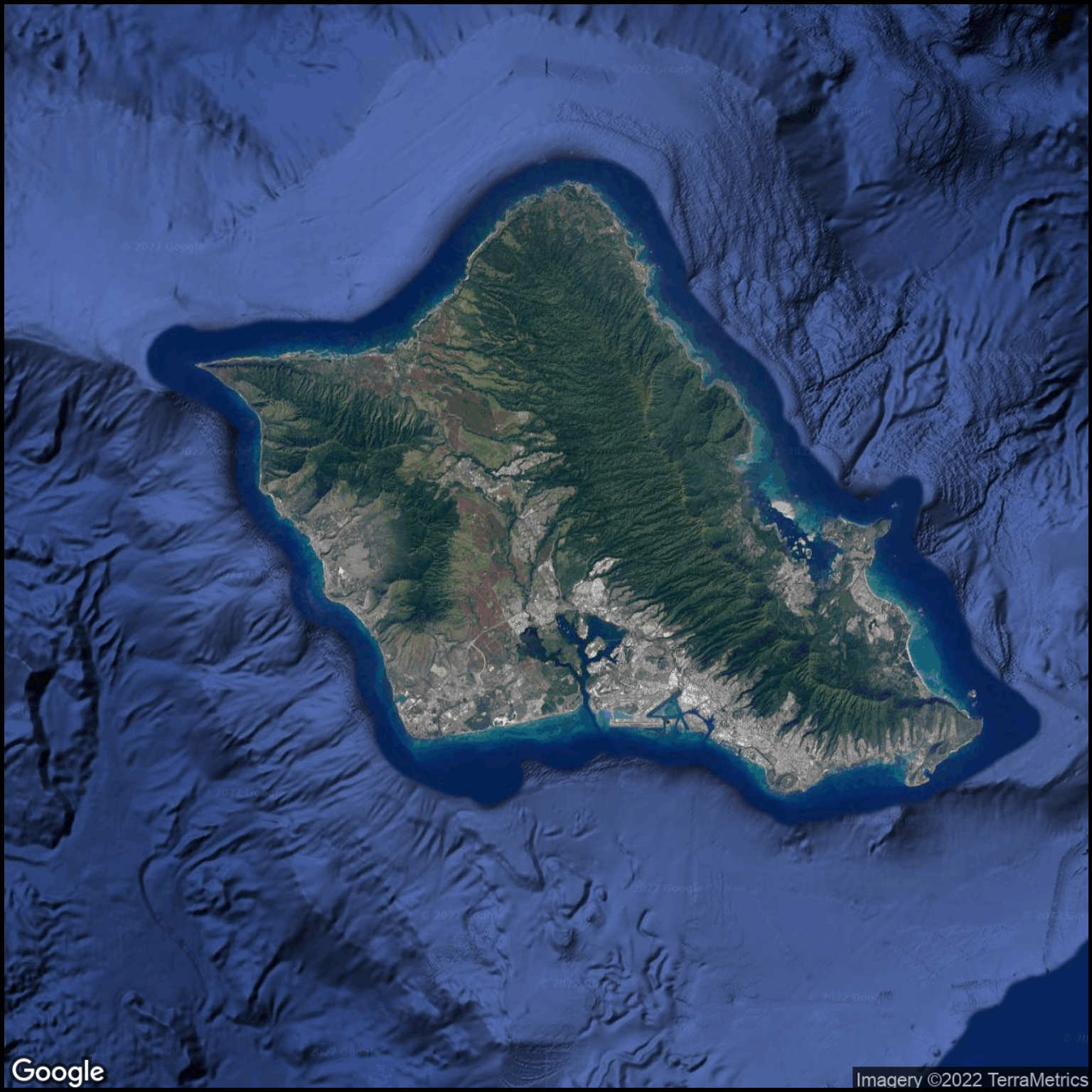
satellite
Satellite image
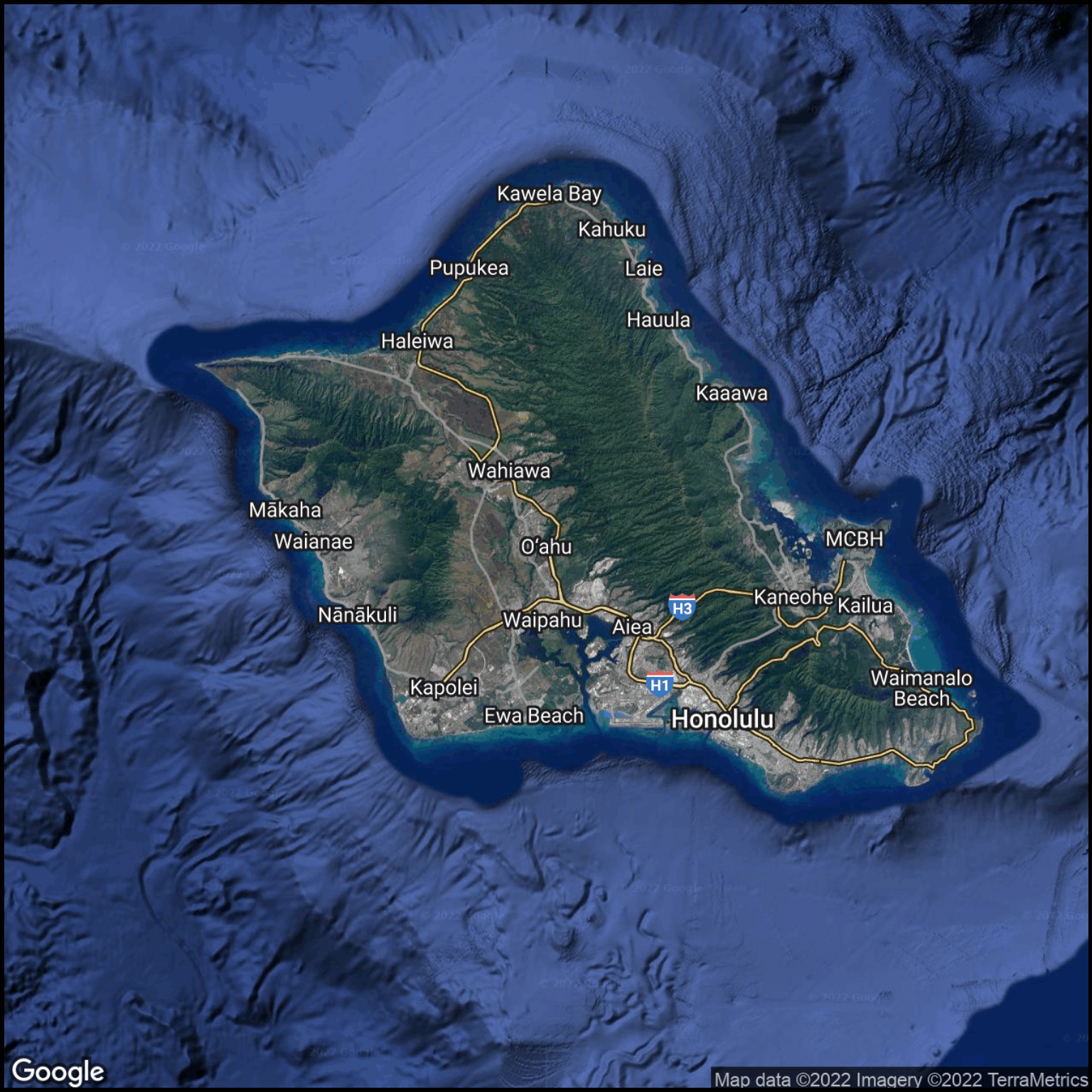
hybrid
Satellite image and street map
Here are a few examples that show some of the types of base maps. Note that the theme (“simple_black_box”), defined earlier, is used to simplify these maps.
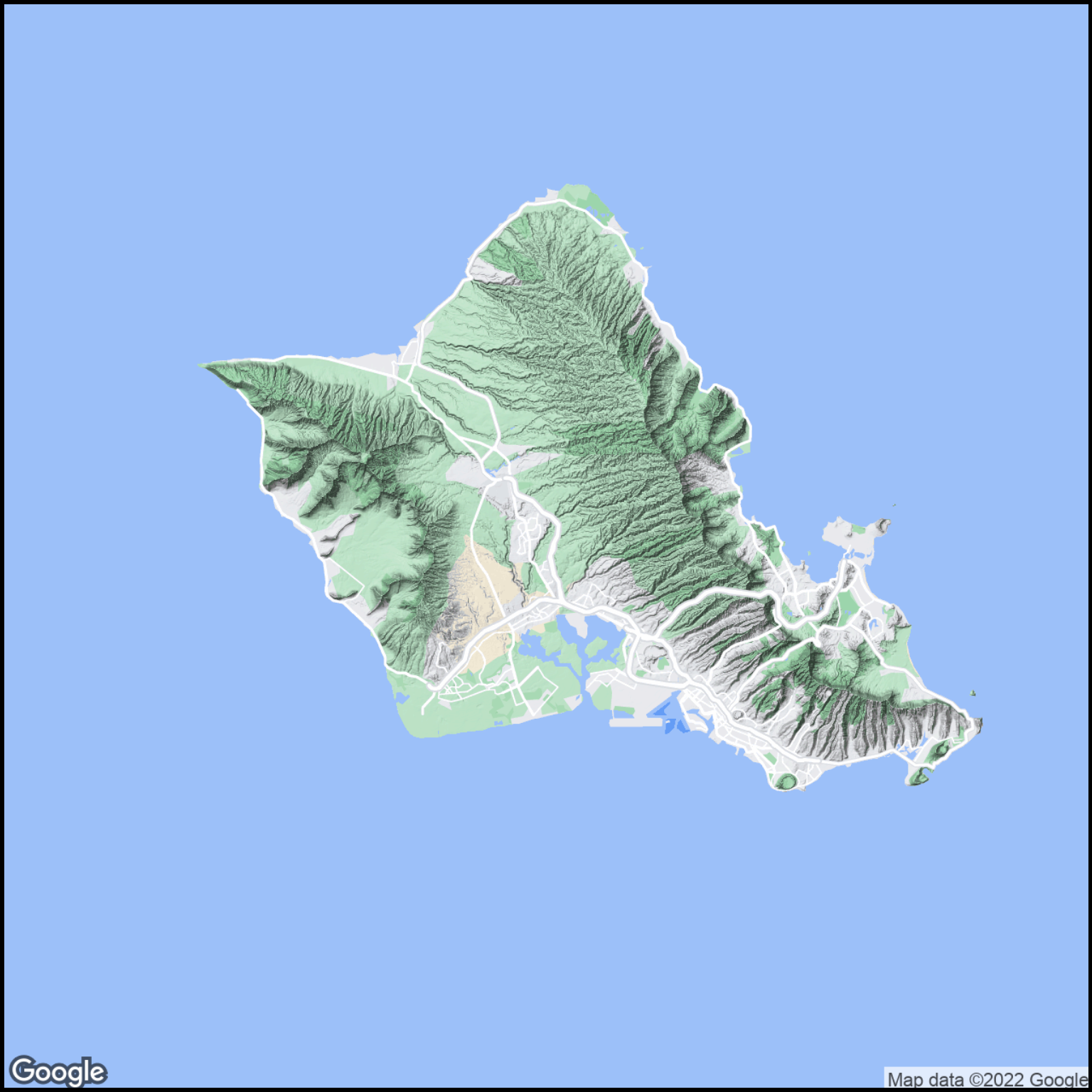
It is possible to “hide” different layers of annotations on Google Maps. This example (Figure 5), which shows the hide$all parameter is just one possibility. See the Google Maps Simplified section for examples of alternative layer hiding.
Figure 5: Oahu, Hawaii as a terrain map with layers hidden.
Scale Differences with Google Maps
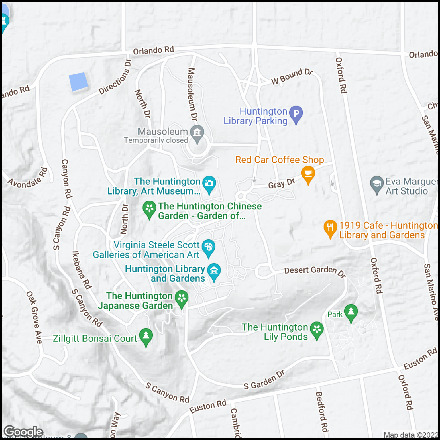
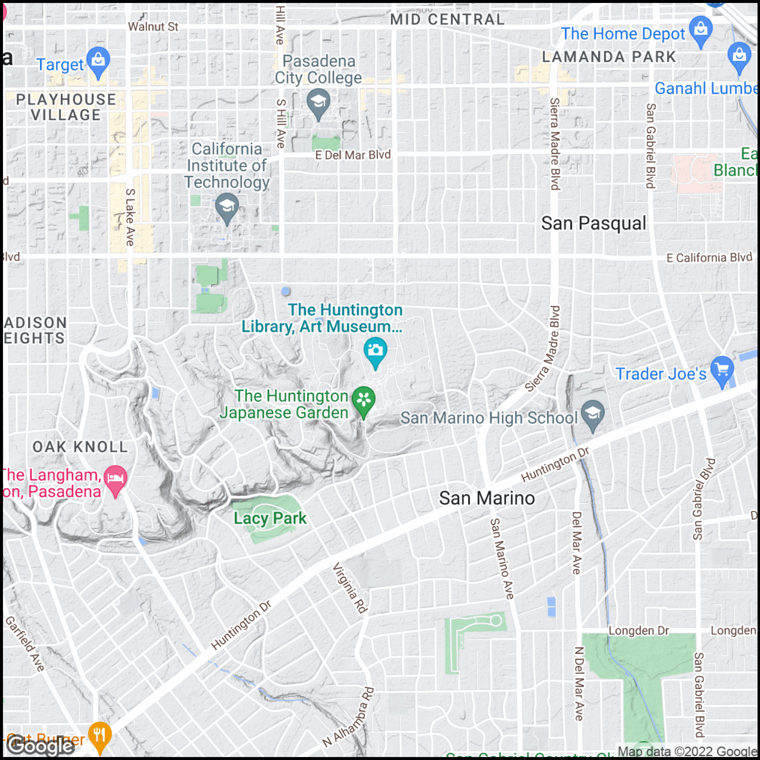
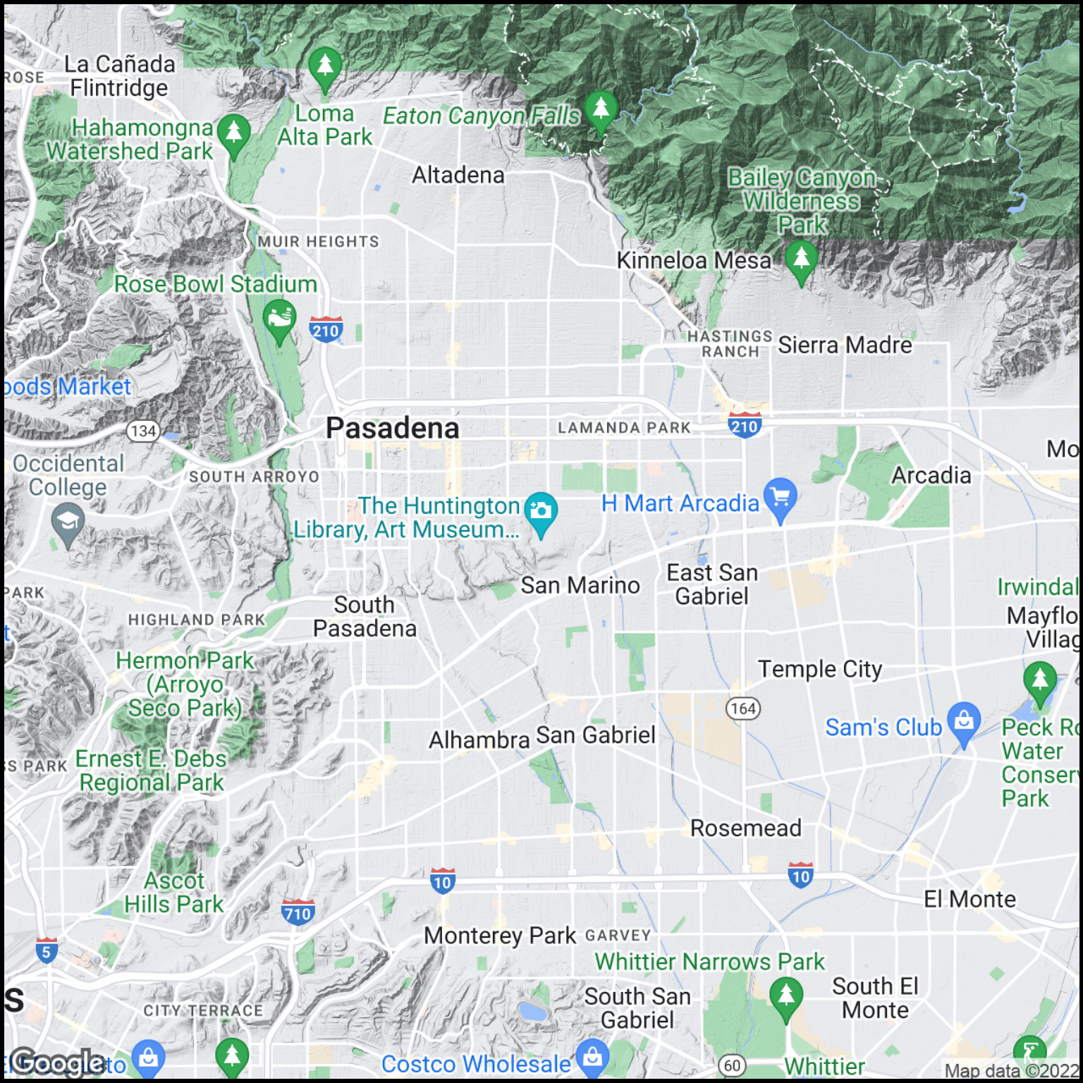
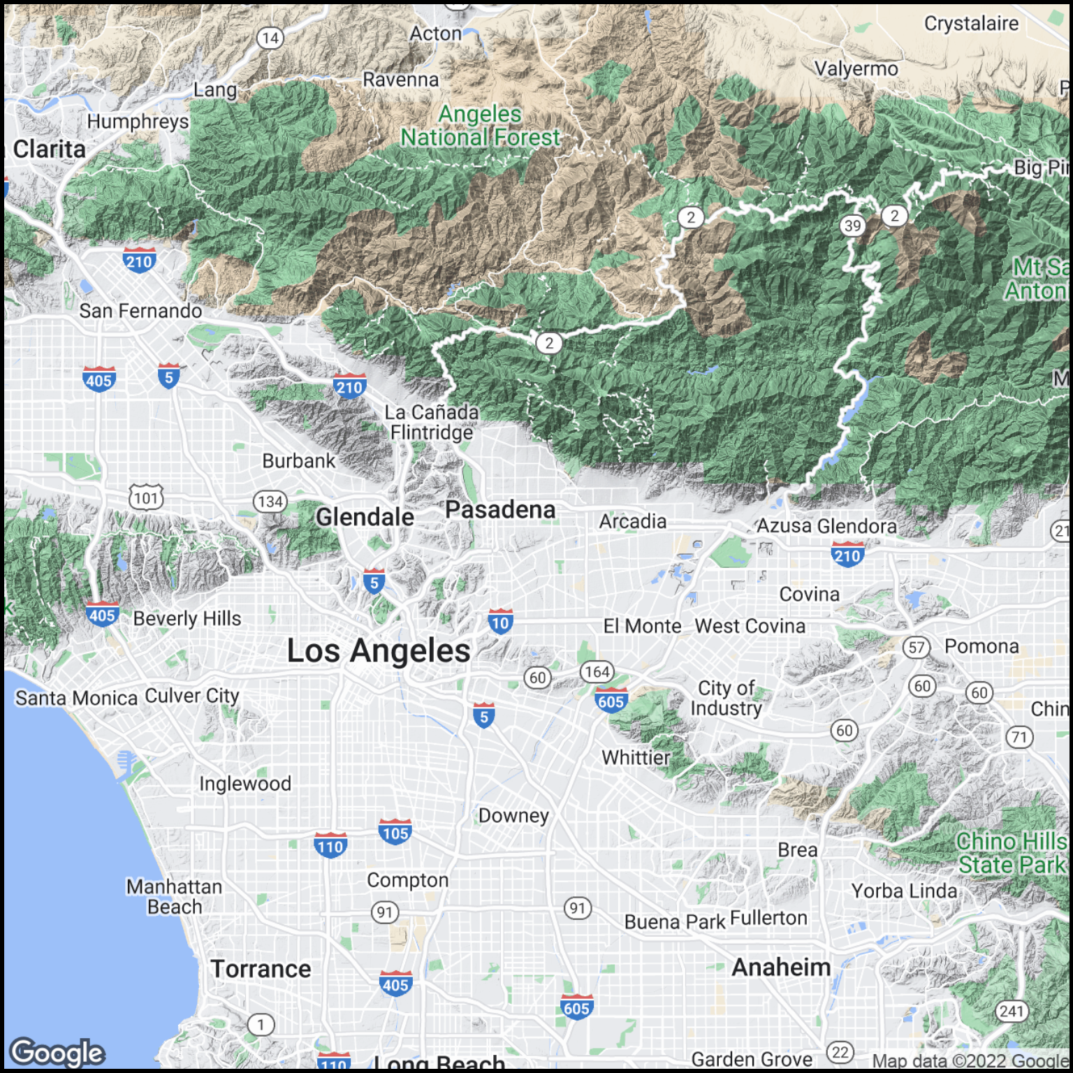
The large property shown in this example (Figure 6) houses the Huntington Library, Art Gallery and Botanical Garden. Zooming out, you see the surrounding neighborhood (Figure 7) and, with even more zoom, the city is shown (Figure 8) next to the adjacent mountains. Finally (Figure 9) you see much of the Los Angeles basin. The original site is now too small to be seen.
These maps give a lot of options when you’re choosing a basemap.
Adding Place Names (preview)
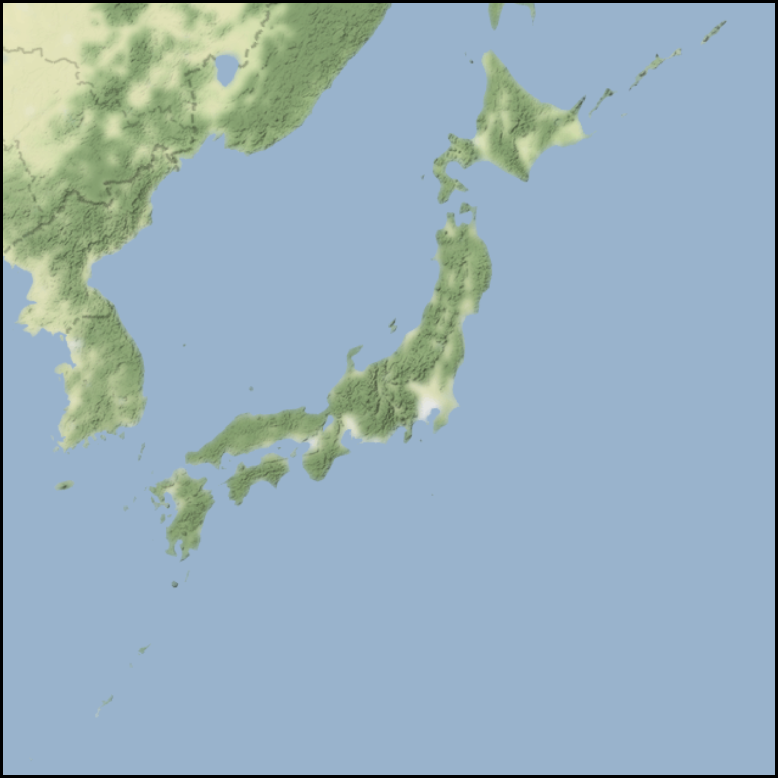
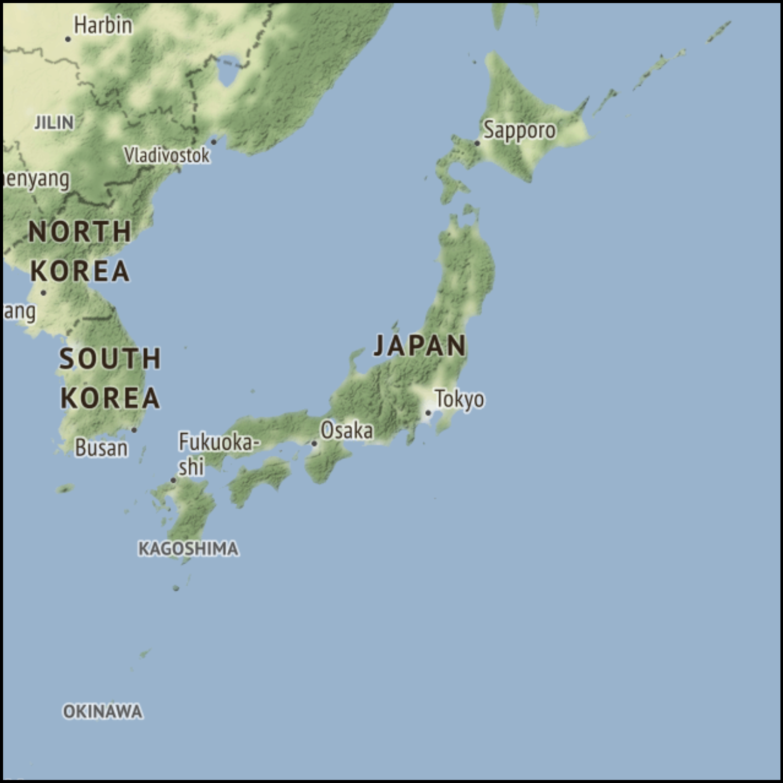
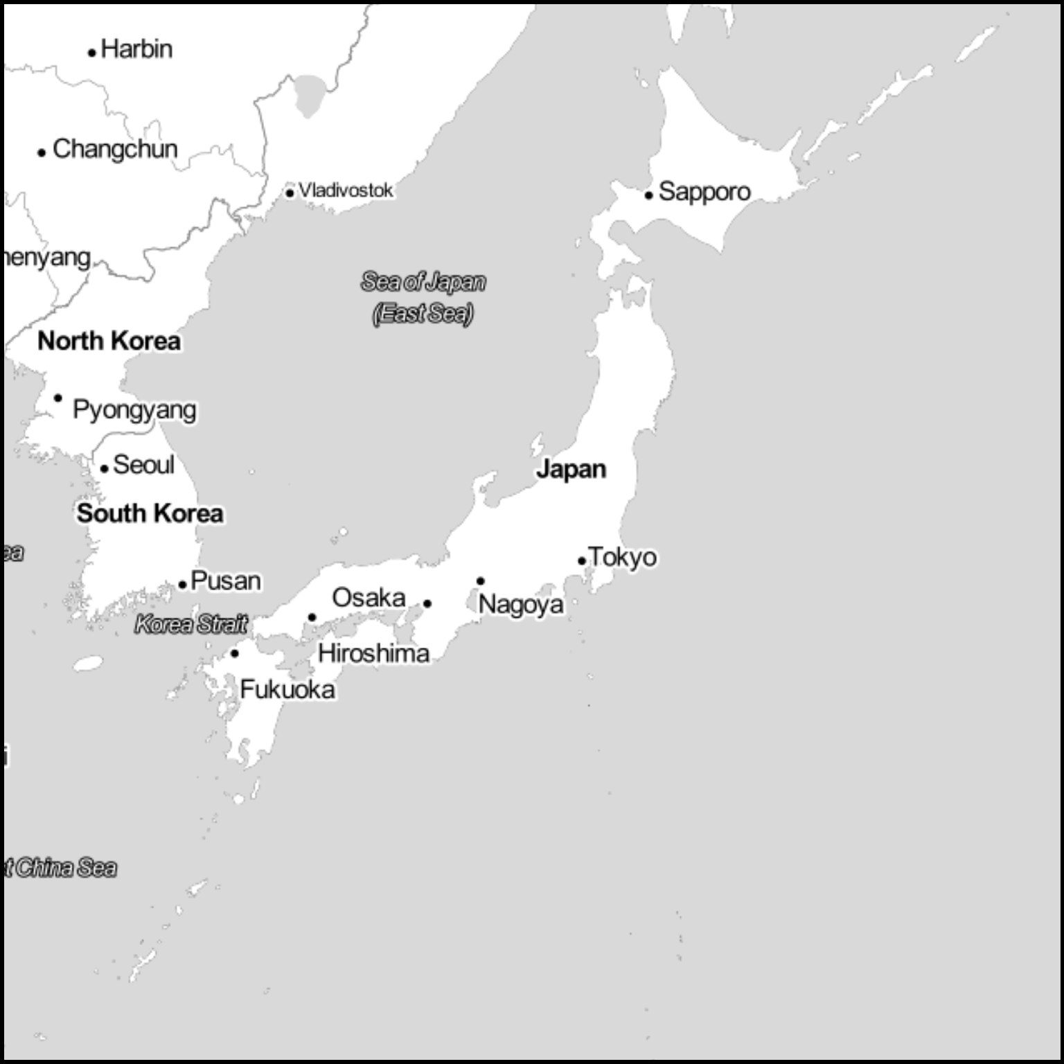
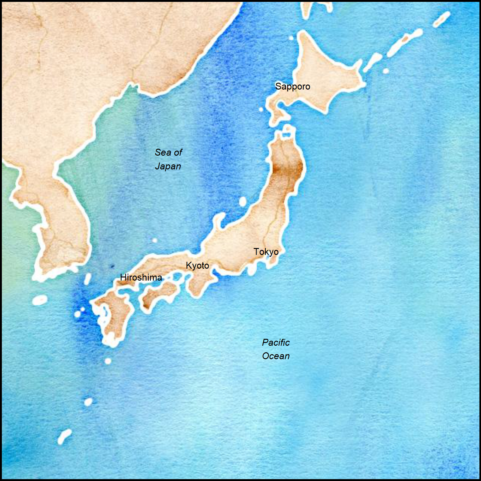
Maps that don’t have names can be given the place names you want. This is an important part of the process in creating a custom map that best serves your visualization requirements.
There is a detailed treatment giving names in a later chapter (Chapter 6: Names). Here is a simple demonstration (Figure 16) that uses the last map (Figure 15).
You can see (in the code) that the names are provided in a table along with coordinate locations and a few style parameters. How these column values work will be explained later.