Google Earth provides an alternative basemap. You get a very flexible system with which to view the terrain, including a number of data overlays. But it is the 3D surface that is the real point of using Google Earth. If the visualization involves complex topography, it might be best to use Google Earth as a basemap.
So, what’s the problem? Google Earth is not “R friendly” the way Google Maps (and Stamen Maps) integrate with the ggplot2 functionality. The workaround is to use R to create an overlay file that will then be imported into Google Earth. The format of such a file is known as “kml” (derived from “keystone markup language,” the precursor to Google Earth.
We’ll get started by doing our usual initialization.
Show the code chunk
library(geosphere)library(sitemaps)library(ggmap)library(ggplot2)library(readr)library(gt)library(dplyr)library(sp) ## To make the SpatialPointslibrary(maptools)## Initialize Google Map key; the key is stored in a Project directory. My_Key <-read_file("P://Hot/Workflow/Workflow/keys/Google_Maps_API_Key.txt")## Test if Google Key is registered.if (!has_google_key()){## Register the Google Maps API Key.register_google(key = My_Key, account_type ="standard") } ## end Google Key test
A few more things.
Show the code chunk
## Use two functions from sitemaps to initialize parameterscolumn <-site_styles()hide <-site_google_hides()## Establish a theme that improves the appearance of a map.## This theme removes the axis labels and ## puts a border around the map. No legend.simple_black_box <-theme_void() +theme(panel.border =element_rect(color ="black", fill=NA, size=2),legend.position ="none")
Example: Colored Points on Google Earth
We’ll reuse some data here. It is the set temperatures in Hawai`i Volcanoes National Park at the Puhimau Hot Spot.
The purpose is to create an overlay (KML data) that can be used with Google Earth.
Note that at this point, we’re not using a Google Earth API to do the overlay. You need to do this part manually by opening Google Earth and opening the kml file that these code chunks create. It is only a matter of time before a “native” R version of a package like RGEE is created. In the meantime, this approach works, even if it doesn’t quite fit into the objective of a reproducible document being entirely recreated when the code is run.
First, let’s get the data ready. There is a data column (color) that is used to for the point colors that will be used on the Google Earth overlay. (This could be created using the site_cut function. But, for simplicity, the colors are simply added as a column here.)
Show the code chunk
## Read in the field data.puhimau <-read_csv(col_names =TRUE, file ="Site, Lon, Lat, Temperature, color 1, -155.251451, 19.389354, 140, red 2, -155.251483, 19.388421, 125, orange 3, -155.249834, 19.389709, 165, red 4, -155.248924, 19.389591, 180, red 5, -155.248982, 19.388827, 102, blue 6, -155.248024, 19.389952, 97, blue 7, -155.249994, 19.388816, 135, orange 8, -155.251831, 19.387395, 95, blue")## Rename the site column and shift all the column names to lowercasepuhimau2 <- puhimau %>% dplyr::rename(text = Site) %>% dplyr::rename_with(tolower)## Show the data in a tablegt(puhimau2) %>%fmt_number(columns =c(lat,lon), decimals =5) %>%tab_source_note(source_note ="Data: 2017 field survey") %>%tab_footnote(footnote ="degrees F",locations =cells_column_labels(columns = temperature))
Table 1: Surface soil temperature measurements at Puhimau Hot Spot.
text
lon
lat
temperature1
color
1
−155.25145
19.38935
140
red
2
−155.25148
19.38842
125
orange
3
−155.24983
19.38971
165
red
4
−155.24892
19.38959
180
red
5
−155.24898
19.38883
102
blue
6
−155.24802
19.38995
97
blue
7
−155.24999
19.38882
135
orange
8
−155.25183
19.38740
95
blue
Data: 2017 field survey
1 degrees F
Now we’re ready to create the Google Earth overlay.
Transform the location data: There is a step where locations are converted to a SpatialPoints data structure. Then, this structure is made into a SpatialPointsDataFrame. In doing this, the puhimau$Temperature column was used pretty much as a dummy element so the conversion would work.
Color symbols as icons: This is a step where small PNG files are created, one for each color point. These need to be persistent data points as the kml overlay will use these when creating the Google Earth image with a data overlay.
The colors come from a column in the data. Because the name of the color is used as part of the PNG file name, you should use only named colors. There are a lot of choices (!) so this should not be a significant limitation.
There are example of the kmlPoints function that use a single icon as the marker symbol. That’s a serious limitation and this example shows that there is at least some increased utility by allowing the markers to have different colors.
Add icon file names to the data: A lookup table is created that lets us merge the names of the colored point icons to the color names in the data.
Create the overlay file: The next step is to build a kml overlay file with the kmlPoints function.
Show the code chunk
## Prepare for Google Earth KLMs_points <-SpatialPoints(coords =cbind(puhimau$Lon,puhimau$Lat))df <-data.frame(puhimau$Temperature)s_points_df <-SpatialPointsDataFrame(s_points,data=df)## Generate PNG icons for use with Google Earth## Get a set of all the colors usedunique_colors <-unique(puhimau$color)number_of_colors <-length(unique_colors)## Initialize a color lookup tablecolor_table <-data.frame(matrix(ncol=2))colnames(color_table) <-c("color","color_file")## Initialize a data frame (which is actually a dummy variable)df <-data.frame(x=2,y=2)for(i in1:number_of_colors){ color <- unique_colors[[i]] p <-ggplot(df,aes(x=2,y=2)) +geom_point(shape =21, color ="black", fill = color, size =30, stroke =3) +theme_void() color_file <-paste0("point_",color,".png")ggsave(p, filename=color_file, dpi=72, width =1, height =1, bg ="transparent")## Add to the color lookup table color_combo <-c(color, color_file) color_table <-rbind(color_table, color_combo) } ## Merge the PNG file names to the data tablepuhimau2 <-merge(puhimau, color_table, by="color")## Create the kml overlay filekmlPoints(obj=s_points_df, kmlfile="KML_test.kml", name = puhimau2$Site,icon = puhimau2$color_file)
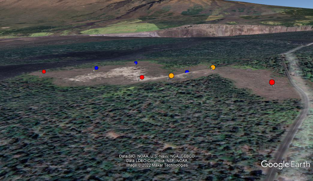
Overlay the kml file in Google Earth: Using the kml file requires that you start Google Earth. Then choose file > open… and select the kml overlay file.
Remember that this process requires the use of the color point icons that you just created.
Screen capture from Google Earth Pro.
What Remains
It will be better when the last step (separately running Google Earth) is integrated into a regular R chunk. That will happen sometime. And it would be nice if Google Earth could be treated just like a Google Maps basemap. Then we would have control over more properties of the point and labels.